Code
x <- seq(-6, 6, length.out = 1000)
plot(x, dcauchy(x, location = 0, scale = 1),
     type = "l", lwd = 3, col = "#2166AC",
     xlab = "x", ylab = "Density",
     main = "PDF of Cauchy(0, 1)", bty = "l")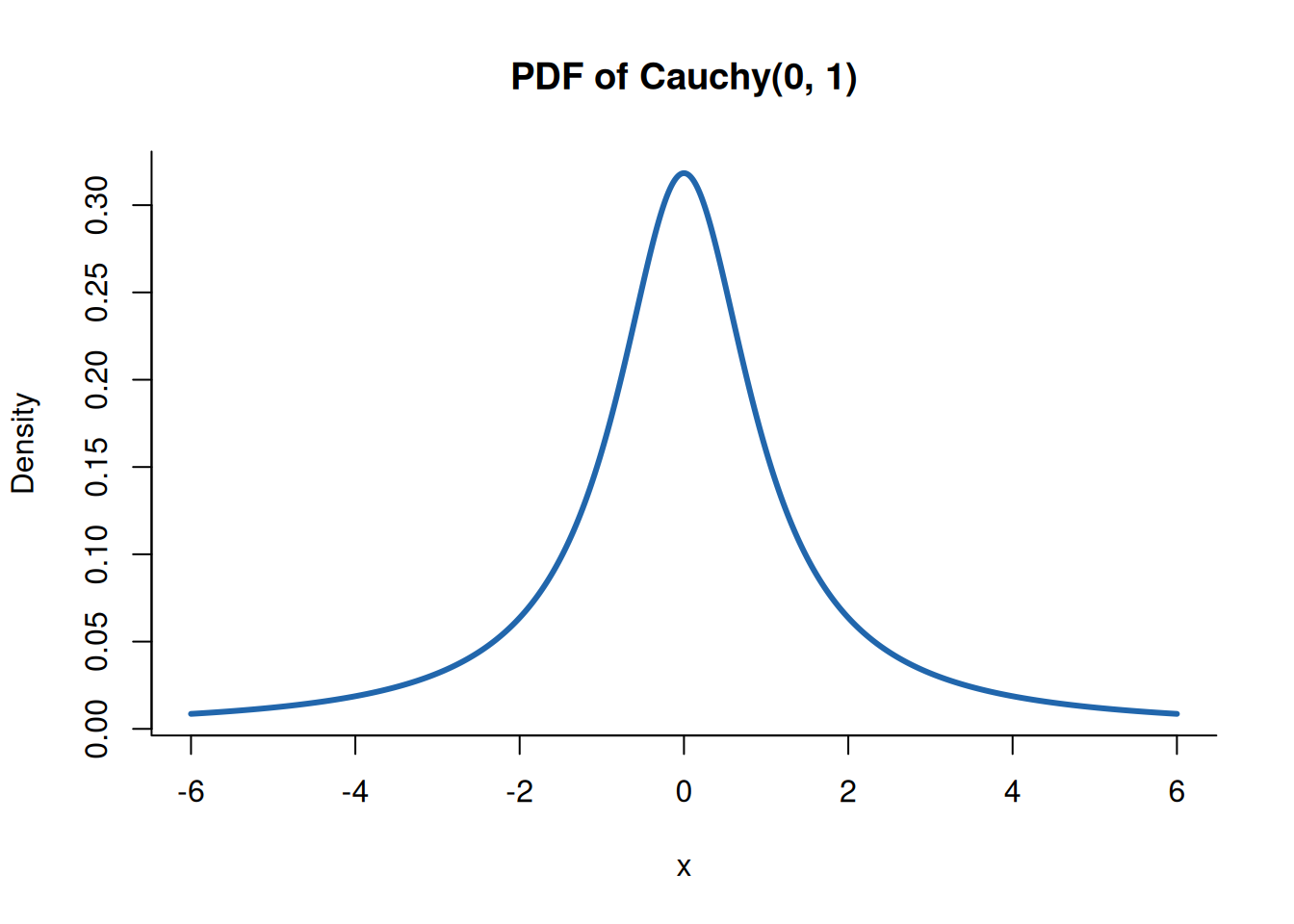
The expected value page required an absolute sum or integral. Why do we need that condition when a symmetric distribution appears to balance perfectly around its center? The Cauchy family gives a case in which the visual center exists but the probability-weighted mean does not.
For x_0\in\mathbb R and \gamma>0, write
X\sim\operatorname{Cauchy}(x_0,\gamma)
when X has density
f_X(x) \equiv \frac{1}{\pi\gamma \left[1+\left(\frac{x-x_0}{\gamma}\right)^2\right]}, \qquad x\in\mathbb R.
The standard Cauchy distribution has x_0=0 and \gamma=1.
x <- seq(-6, 6, length.out = 1000)
plot(x, dcauchy(x, location = 0, scale = 1),
type = "l", lwd = 3, col = "#2166AC",
xlab = "x", ylab = "Density",
main = "PDF of Cauchy(0, 1)", bty = "l")
The density is symmetric around zero, so the tempting move is to pair each positive contribution with a negative one and declare the mean zero. The next calculation shows why that move is not licensed.
For the standard Cauchy density,
x f_X(x)=\frac{x}{\pi(1+x^2)}.
Consider the positive part:
\begin{aligned} \int_0^b \frac{x}{\pi(1+x^2)}\,\mathrm dx &=\frac{1}{2\pi}\log(1+b^2). \end{aligned}
As b\to\infty, this quantity diverges to +\infty. By symmetry, the integral over the negative half-line diverges to -\infty. An expectation exists only when these two parts can be combined without making the result depend on how the limits are taken. Here they cannot, so
\mathbb E[X]
is undefined.
For every finite b>0,
\int_{-b}^{b}x f_X(x)\,\mathrm dx=0.
Taking the symmetric limit produces a Cauchy principal value of zero. An expectation is not defined by forcing the positive and negative truncation bounds to approach infinity at the same rate. It requires the probability-weighted integral itself to exist. Thus the principal value is not \mathbb E[X].
Every finite sample of Cauchy draws has a finite arithmetic mean, but that fact does not imply that the distribution has an expected value. As the sample grows, an extreme draw can move the sample mean by an arbitrarily large amount. The model supplies no finite population mean to which those sample means must converge.
The exact upshot is that symmetry identifies a geometric center but does not guarantee a finite expected value. The later summaries in this module, including variance, likewise require their defining expectations to exist.