The preceding pages introduced continuous distributions through their probability density functions. Suppose a phonetic model represents an F_1 measurement as varying symmetrically around 550 Hz. The density is highest at 550 and decreases as distance from 550 increases in either direction. Which parameters let us move the center and spread separately while preserving this symmetric shape?
F_1 is an acoustic formant measurement. Classic vowel research relates formant measurements, produced vowel categories, and listener identifications while keeping those objects distinct (Peterson and Barney 1952). A normal model for F_1 can represent measured variation, but one F_1 value does not by itself determine a phonological category or percept.
The normal distribution is a continuous location and scale family with this symmetric shape. Its two parameters answer the location and spread questions. We write
X\sim\mathcal{N}(\mu,\sigma^2).
The first parameter is the mean:
\mathbb{E}[X]=\mu.
The second parameter is the variance:
\operatorname{Var}(X)=\sigma^2.
Thus \mu sets location, while \sigma sets scale. The standard deviation is \sigma, not the second written parameter \sigma^2.
At x=\mu, the centered distance x-\mu is zero, so the density reaches its maximum. Moving the same distance above or below \mu produces the same squared distance and thus the same density.
This equality gives the family’s symmetry:
f_X(\mu-d)=f_X(\mu+d).
The density decreases smoothly as |d| grows.
Changing location while holding scale fixed
Increasing \mu shifts the full density to larger values, whereas decreasing \mu shifts it to smaller values. The spread and symmetric shape remain unchanged when \sigma is held fixed.
For instance, moving from \mathcal{N}(550,40^2) to \mathcal{N}(600,40^2) adds 50 Hz to the center without changing the standard deviation.
Changing scale while holding location fixed
Increasing \sigma spreads probability across a wider range and lowers the density peak because the total area must remain one, whereas decreasing \sigma concentrates probability nearer \mu.
Compare \mathcal{N}(550,40^2) with \mathcal{N}(550,80^2). Both have mean 550 Hz, but the second standard deviation is twice as large.
Code
f1 <-seq(300, 800, length.out =400)plot(f1, dnorm(f1, mean =550, sd =40), type ="l",xlab =expression(F[1]~"in Hz"), ylab ="density")lines(f1, dnorm(f1, mean =600, sd =40), lty =2)lines(f1, dnorm(f1, mean =550, sd =80), lty =3)
The first comparison isolates location; the second isolates scale.
Comparing location and scale
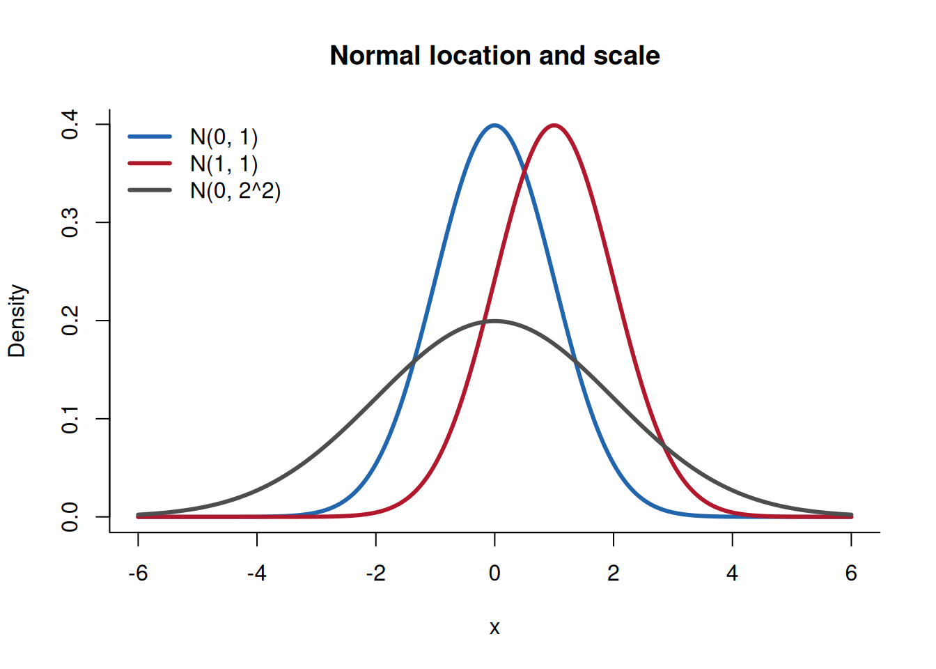
The original sequence compares a standard normal density with a location shift and a scale increase. The third label below is \mathcal N(0,2^2) because R’s sd argument is a standard deviation, while the second mathematical parameter is a variance.
pnorm(590, mean =550, sd =40) -pnorm(510, mean =550, sd =40)
This interval calculation is a property of the normal family. It is not a universal rule for every distribution with mean 550 and standard deviation 40.
A normal variable has support across the full real line. It assigns some density to negative values even when the measurement, such as F_1, cannot be negative.
The approximation may still be useful when the mean is many standard deviations from the boundary and the modeled density below zero is negligible. It may be poor for a strongly right skewed response or one concentrated near a hard boundary.
A histogram is not enough
A roughly bell shaped histogram does not by itself justify a normal model. A finite histogram may hide tail asymmetry, boundary problems, or repeated structure across speakers and items.
Check the support, the symmetry claim, and the deviations relevant to the linguistic analysis. Visual familiarity alone does not establish those properties.
Check your understanding
In \mathcal{N}(100,225), what are the mean, variance, and standard deviation?
Standardize X=130 under the model in the first question.
Which parameter changes when a density shifts right without changing shape?
Give one linguistic response for which support on the full real line may be a poor direct choice.
---title: "The normal distribution"execute: enabled: true echo: true warning: false message: false---The preceding pages introduced continuous distributions through their [probability density functions](probability-density-functions.qmd). Suppose a phonetic model represents an $F_1$ measurement as varying symmetrically around 550 Hz. The density is highest at 550 and decreases as distance from 550 increases in either direction. Which parameters let us move the center and spread separately while preserving this symmetric shape?$F_1$ is an acoustic formant measurement. Classic vowel research relates formant measurements, produced vowel categories, and listener identifications while keeping those objects distinct ([Peterson and Barney 1952](https://doi.org/10.1121/1.1906875)). A normal model for $F_1$ can represent measured variation, but one $F_1$ value does not by itself determine a phonological category or percept.The [**normal distribution**](https://bruno.nicenboim.me/bayescogsci/ch-intro.html) is a continuous location and scale family with this symmetric shape. Its two parameters answer the location and spread questions. We write$$X\sim\mathcal{N}(\mu,\sigma^2).$$The first parameter is the mean:$$\mathbb{E}[X]=\mu.$$The second parameter is the variance:$$\operatorname{Var}(X)=\sigma^2.$$Thus $\mu$ sets location, while $\sigma$ sets scale. The standard deviation is $\sigma$, not the second written parameter $\sigma^2$.## Reading the density from the center outwardThe density is$$f_X(x)\equiv\frac{1}{\sqrt{2\pi\sigma^2}} \exp\!\left[-\frac{(x-\mu)^2}{2\sigma^2}\right].$$At $x=\mu$, the centered distance $x-\mu$ is zero, so the density reaches its maximum. Moving the same distance above or below $\mu$ produces the same squared distance and thus the same density.This equality gives the family's symmetry:$$f_X(\mu-d)=f_X(\mu+d).$$The density decreases smoothly as $|d|$ grows.## Changing location while holding scale fixedIncreasing $\mu$ shifts the full density to larger values, whereas decreasing $\mu$ shifts it to smaller values. The spread and symmetric shape remain unchanged when $\sigma$ is held fixed.For instance, moving from $\mathcal{N}(550,40^2)$ to $\mathcal{N}(600,40^2)$ adds 50 Hz to the center without changing the standard deviation.## Changing scale while holding location fixedIncreasing $\sigma$ spreads probability across a wider range and lowers the density peak because the total area must remain one, whereas decreasing $\sigma$ concentrates probability nearer $\mu$.Compare $\mathcal{N}(550,40^2)$ with $\mathcal{N}(550,80^2)$. Both have mean 550 Hz, but the second standard deviation is twice as large.```{r}#| eval: falsef1 <-seq(300, 800, length.out =400)plot(f1, dnorm(f1, mean =550, sd =40), type ="l",xlab =expression(F[1]~"in Hz"), ylab ="density")lines(f1, dnorm(f1, mean =600, sd =40), lty =2)lines(f1, dnorm(f1, mean =550, sd =80), lty =3)```The first comparison isolates location; the second isolates scale.## Comparing location and scaleThe original sequence compares a standard normal density with a location shift and a scale increase. The third label below is $\mathcal N(0,2^2)$ because R's `sd` argument is a standard deviation, while the second mathematical parameter is a variance.```{r}x_normal <-seq(-6, 6, length.out =1000)plot(x_normal, dnorm(x_normal, 0, 1), type ="l", lwd =3,col ="#2166AC", xlab ="x", ylab ="Density",main ="Normal location and scale", bty ="l")lines(x_normal, dnorm(x_normal, 1, 1), lwd =3, col ="#B2182B")lines(x_normal, dnorm(x_normal, 0, 2), lwd =3, col ="#4D4D4D")legend("topleft", c("N(0, 1)", "N(1, 1)", "N(0, 2^2)"),col =c("#2166AC", "#B2182B", "#4D4D4D"),lty =1, lwd =3, bty ="n")```The mean changes location. The standard deviation changes scale.## Standardizing one value[**Standardization**](https://appliedstatisticsforlinguists.org/bwinter_stats_proofs.pdf#page=102) subtracts the mean and divides by the standard deviation. The resulting [**z-score**](https://openstax.org/books/introductory-statistics-2e/pages/6-1-the-standard-normal-distribution)$$Z\equiv\frac{X-\mu}{\sigma}$$records signed distance from the mean in standard deviation units. Under the normal model,$$Z\sim\mathcal{N}(0,1).$$For $X\sim\mathcal{N}(550,40^2)$, the values 510 and 590 are one standard deviation below and above the mean:$$\frac{510-550}{40}=-1$$and$$\frac{590-550}{40}=1.$$The probability between them is$$\mathbb{P}(510\leq X\leq590)=\mathbb{P}(-1\leq Z\leq1)\approx.683.$$In R,```{r}#| eval: falsepnorm(590, mean =550, sd =40) -pnorm(510, mean =550, sd =40)```This interval calculation is a property of the normal family. It is not a universal rule for every distribution with mean 550 and standard deviation 40.## Comparing CDFsFor a standard normal random variable,$$\Phi(x)\equiv\mathbb P(X\leq x)=\int_{-\infty}^{x}\frac{1}{\sqrt{2\pi}}e^{-t^2/2}\,\mathrm dt.$$```{r}plot(x_normal, pnorm(x_normal), type ="l", lwd =3, col ="#2166AC",xlab ="x", ylab ="Cumulative probability",main ="CDF of N(0, 1)", ylim =c(0, 1), bty ="l")```The S shape is not unique to the normal family. Compare it with the CDF of $\operatorname{Beta}(5,5)$.```{r}x_beta <-seq(0, 1, length.out =800)plot(x_beta, pbeta(x_beta, 5, 5), type ="l", lwd =3,col ="#2166AC", xlab ="x", ylab ="Cumulative probability",main ="CDF of Beta(5, 5)", ylim =c(0, 1), bty ="l")```## Checking support against the measurementA normal variable has support across the full real line. It assigns some density to negative values even when the measurement, such as $F_1$, cannot be negative.The approximation may still be useful when the mean is many standard deviations from the boundary and the modeled density below zero is negligible. It may be poor for a strongly right skewed response or one concentrated near a hard boundary.## A histogram is not enoughA roughly bell shaped histogram does not by itself justify a normal model. A finite histogram may hide tail asymmetry, boundary problems, or repeated structure across speakers and items.Check the support, the symmetry claim, and the deviations relevant to the linguistic analysis. Visual familiarity alone does not establish those properties.## Check your understanding1. In $\mathcal{N}(100,225)$, what are the mean, variance, and standard deviation?2. Standardize $X=130$ under the model in the first question.3. Which parameter changes when a density shifts right without changing shape?4. Give one linguistic response for which support on the full real line may be a poor direct choice.The normal family supplies the standard normal variables used to construct the [chi-squared distribution on the next page](chi-squared-distribution.qmd).