Suppose a sampled token must receive exactly one label from a finite inventory. How do we specify a distribution when the possible values are names such as pronouns rather than numerical measurements? Use the case-coded English pronouns
This list answers the first question by declaring the support. The ordering is part of the parameterization because it fixes which probability belongs to which pronoun label.
The split copies of you and it represent case-annotated tokens, not distinct surface word types. This follows the Universal Dependencies English case convention, under which these forms may receive nominative or accusative case according to their syntactic context.
Definition
Basically, a categorical distribution pairs each label with one probability. More specifically, a categorical distribution assigns probability to a finite set of labels. Let R record pronoun identity and take values in \mathcal V\equiv\{v_1,\ldots,v_K\}. For a vector
\boldsymbol\pi\equiv(\pi_1,\ldots,\pi_K)
such that \pi_k\geq0 and \sum_{k=1}^K\pi_k=1, we write
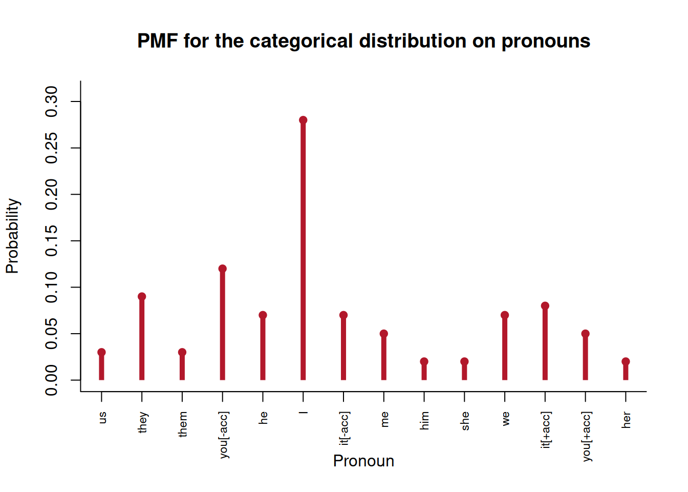
plot(seq_along(pronoun_probability), pronoun_probability,type ="h", lwd =5, lend =1, col ="#B2182B",xaxt ="n", xlab ="Pronoun", ylab ="Probability",main ="PMF for the categorical distribution on pronouns",ylim =c(0, .31), bty ="l")axis(1, at =seq_along(pronoun_probability),labels =names(pronoun_probability), las =2, cex.axis = .72)points(seq_along(pronoun_probability), pronoun_probability,pch =19, col ="#B2182B")
The graph is the PMF evaluated at all fourteen pronoun values. Its vertical coordinates are probabilities, not densities.
Label order
Suppose a permutation sends v_k to position j. The same permutation must send \pi_k to position j. Reordering the labels while holding the numeric vector fixed assigns the probabilities to different pronouns and thus defines a different distribution.
The labels themselves need not be numerical or ordered. The integer position merely indexes the corresponding entry of \boldsymbol\pi.
Check your understanding
Verify that the displayed probability vector sums to one.
State p_R(\textit{I}) and p_R(\textit{her}).
Explain why permuting only the labels changes the distribution.
State how many free probabilities remain after fixing the support size at K.
The Bernoulli distribution is the categorical special case with two values coded as zero and one.
Source Code
---title: "The categorical distribution"execute: enabled: true echo: true warning: false message: false---Suppose a sampled token must receive exactly one label from a finite inventory. How do we specify a distribution when the possible values are names such as pronouns rather than numerical measurements? Use the case-coded English pronouns$$\begin{aligned}\mathcal V\equiv(&\textit{us},\textit{they},\textit{them},\textit{you}_{[-\mathrm{acc}]},\textit{he},\textit{I},\textit{it}_{[-\mathrm{acc}]},\textit{me},\textit{him},\textit{she},\\&\textit{we},\textit{it}_{[+\mathrm{acc}]},\textit{you}_{[+\mathrm{acc}]},\textit{her}).\end{aligned}$$This list answers the first question by declaring the support. The ordering is part of the parameterization because it fixes which probability belongs to which pronoun label.The split copies of *you* and *it* represent case-annotated tokens, not distinct surface word types. This follows the [Universal Dependencies English case convention](https://universaldependencies.org/docsv1/en/feat/Case.html), under which these forms may receive nominative or accusative case according to their syntactic context.## DefinitionBasically, a categorical distribution pairs each label with one probability. More specifically, a [**categorical distribution**](https://mc-stan.org/docs/functions-reference/categorical-distribution.html) assigns probability to a finite set of labels. Let $R$ record pronoun identity and take values in $\mathcal V\equiv\{v_1,\ldots,v_K\}$. For a vector$$\boldsymbol\pi\equiv(\pi_1,\ldots,\pi_K)$$such that $\pi_k\geq0$ and $\sum_{k=1}^K\pi_k=1$, we write$$R\sim\operatorname{Categorical}(\boldsymbol\pi)$$when$$p_R(v_k)\equiv\mathbb P(R=v_k)=\pi_k,\qquad k\in\{1,\ldots,K\}.$$The symbol $\sim$ means “is distributed as.” It is not an equality between the random variable and the probability vector.## The pronoun exampleDefine the probability vector$$\boldsymbol\pi\equiv(.03,.09,.03,.12,.07,.28,.07,.05,.02,.02,.07,.08,.05,.02).$$The first probability belongs to *us*, the second to *they*, and so on through the ordered list $\mathcal V$. The probabilities sum to one.```{r}pronoun_probability <-c(us = .03,they = .09,them = .03,`you[-acc]`= .12,he = .07,I = .28,`it[-acc]`= .07,me = .05,him = .02,she = .02,we = .07,`it[+acc]`= .08,`you[+acc]`= .05,her = .02)sum(pronoun_probability)plot(seq_along(pronoun_probability), pronoun_probability,type ="h", lwd =5, lend =1, col ="#B2182B",xaxt ="n", xlab ="Pronoun", ylab ="Probability",main ="PMF for the categorical distribution on pronouns",ylim =c(0, .31), bty ="l")axis(1, at =seq_along(pronoun_probability),labels =names(pronoun_probability), las =2, cex.axis = .72)points(seq_along(pronoun_probability), pronoun_probability,pch =19, col ="#B2182B")```The graph is the PMF evaluated at all fourteen pronoun values. Its vertical coordinates are probabilities, not densities.## Label orderSuppose a permutation sends $v_k$ to position $j$. The same permutation must send $\pi_k$ to position $j$. Reordering the labels while holding the numeric vector fixed assigns the probabilities to different pronouns and thus defines a different distribution.The labels themselves need not be numerical or ordered. The integer position merely indexes the corresponding entry of $\boldsymbol\pi$.## Check your understanding1. Verify that the displayed probability vector sums to one.2. State $p_R(\textit{I})$ and $p_R(\textit{her})$.3. Explain why permuting only the labels changes the distribution.4. State how many free probabilities remain after fixing the support size at $K$.The [Bernoulli distribution](bernoulli-distribution.qmd) is the categorical special case with two values coded as zero and one.