The categorical distribution permits any finite support. What changes when the scientific question divides those outcomes into just two classes, target and nontarget? The Bernoulli family represents that binary case.
Return to the case-coded pronoun sample space and define the accusative event
The range of X is \{0,1\} even though the sample space contains fourteen pronoun outcomes. This is the decisive compression: the Bernoulli restriction concerns the random variable’s range, not the size of \Omega.
The binary code presupposes a case annotation for syncretic surface forms such as you and it. The Universal Dependencies English guidelines use syntactic context for that annotation; the surface string alone does not supply it.
Definition
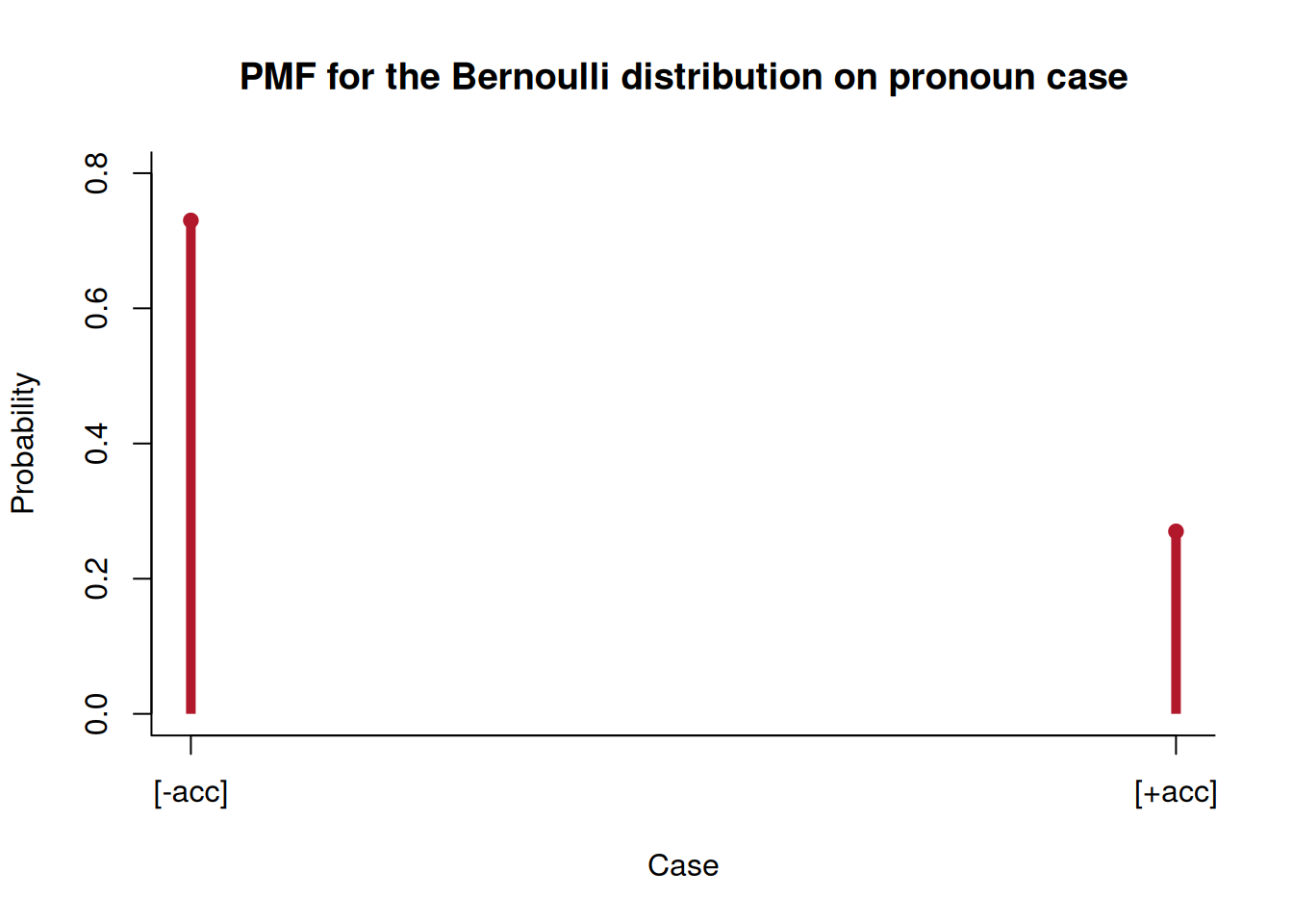
Basically, one parameter records the probability of the event coded as 1, and the remaining probability goes to 0. More specifically, the Bernoulli distribution assigns probability to a binary random variable. For \pi\in[0,1], we write
For \pi=.27, \operatorname{Var}(X)=.27(.73)=.1971.
Why the case coding matters
If the surface forms you and it are not split into case-coded outcomes, a binary case variable is not defined for them without an additional annotation rule. Let A_{12} and N_{12} be the overlapping accusative and nonaccusative events in the twelve-form space. One option is a three-valued variable:
This variable is categorical, not Bernoulli. Alternatively, a pair of indicators can record membership in A_{12} and N_{12} separately.
Check your understanding
Explain why fourteen pronoun outcomes can induce a two-valued Bernoulli variable.
Reverse the coding so that nonaccusative case receives one. State the new Bernoulli parameter.
Derive \mathbb E[X] and \operatorname{Var}(X) from the two PMF values.
Explain why the unsplit surface forms you and it require a nonbinary representation or an additional case annotation.
Source Code
---title: "The Bernoulli distribution"execute: enabled: true echo: true warning: false message: false---The [categorical distribution](bernoulli-and-categorical-distributions.qmd) permits any finite support. What changes when the scientific question divides those outcomes into just two classes, target and nontarget? The Bernoulli family represents that binary case.Return to the case-coded pronoun sample space and define the accusative event$$A_{14}\equiv\{\textit{me},\textit{you}_{[+\mathrm{acc}]},\textit{them},\textit{her},\textit{him},\textit{it}_{[+\mathrm{acc}]},\textit{us}\}.$$Define the indicator random variable$$X(\omega)\equiv\begin{cases}1,&\omega\in A_{14},\\0,&\omega\notin A_{14}.\end{cases}$$The range of $X$ is $\{0,1\}$ even though the sample space contains fourteen pronoun outcomes. This is the decisive compression: the Bernoulli restriction concerns the random variable's range, not the size of $\Omega$.The binary code presupposes a case annotation for syncretic surface forms such as *you* and *it*. The [Universal Dependencies English guidelines](https://universaldependencies.org/docsv1/en/feat/Case.html) use syntactic context for that annotation; the surface string alone does not supply it.## DefinitionBasically, one parameter records the probability of the event coded as 1, and the remaining probability goes to 0. More specifically, the [**Bernoulli distribution**](https://bruno.nicenboim.me/bayescogsci/ch-intro.html) assigns probability to a binary random variable. For $\pi\in[0,1]$, we write$$X\sim\operatorname{Bernoulli}(\pi)$$when$$p_X(x)\equiv\mathbb P(X=x)=\pi^x(1-\pi)^{1-x},\qquad x\in\{0,1\}.$$Substituting the two support values gives$$p_X(1)=\pi\qquad\text{and}\qquadp_X(0)=1-\pi.$$Thus $\pi$ is the probability of the event coded as one. The definition of $X$ makes that event explicit.## The pronoun-case exampleSet $\pi=.27$. Then$$p_X(1)=.27\qquad\text{and}\qquadp_X(0)=.73.$$```{r}case_code <-0:1case_mass <-dbinom(case_code, size =1, prob = .27)plot(case_code, case_mass, type ="h", lwd =5, lend =1,col ="#B2182B", xaxt ="n", xlab ="Case", ylab ="Probability",main ="PMF for the Bernoulli distribution on pronoun case",ylim =c(0, .8), bty ="l")axis(1, at = case_code, labels =c("[-acc]", "[+acc]"))points(case_code, case_mass, pch =19, col ="#B2182B")```## Mean and varianceThe expected value is$$\begin{aligned}\mathbb E[X]&=0(1-\pi)+1(\pi)\\&=\pi.\end{aligned}$$The variance is$$\begin{aligned}\operatorname{Var}(X)&=(0-\pi)^2(1-\pi)+(1-\pi)^2\pi\\&=\pi(1-\pi).\end{aligned}$$For $\pi=.27$, $\operatorname{Var}(X)=.27(.73)=.1971$.## Why the case coding mattersIf the surface forms *you* and *it* are not split into case-coded outcomes, a binary case variable is not defined for them without an additional annotation rule. Let $A_{12}$ and $N_{12}$ be the overlapping accusative and nonaccusative events in the twelve-form space. One option is a three-valued variable:$$C(\omega)\equiv\begin{cases}2,&\omega\in A_{12}\cap N_{12},\\1,&\omega\in A_{12}\setminus N_{12},\\0,&\omega\in N_{12}\setminus A_{12},\end{cases}$$This variable is categorical, not Bernoulli. Alternatively, a pair of indicators can record membership in $A_{12}$ and $N_{12}$ separately.## Check your understanding1. Explain why fourteen pronoun outcomes can induce a two-valued Bernoulli variable.2. Reverse the coding so that nonaccusative case receives one. State the new Bernoulli parameter.3. Derive $\mathbb E[X]$ and $\operatorname{Var}(X)$ from the two PMF values.4. Explain why the unsplit surface forms *you* and *it* require a nonbinary representation or an additional case annotation.