Code
k <- 0:9
mass <- 2^(-(k + 1))
plot(k, mass, type = "h", lwd = 5, lend = 1, col = "#B2182B",
     xlab = "k", ylab = "Probability",
     main = "PMF defined by a geometric series", bty = "l")
points(k, mass, pch = 19, col = "#B2182B")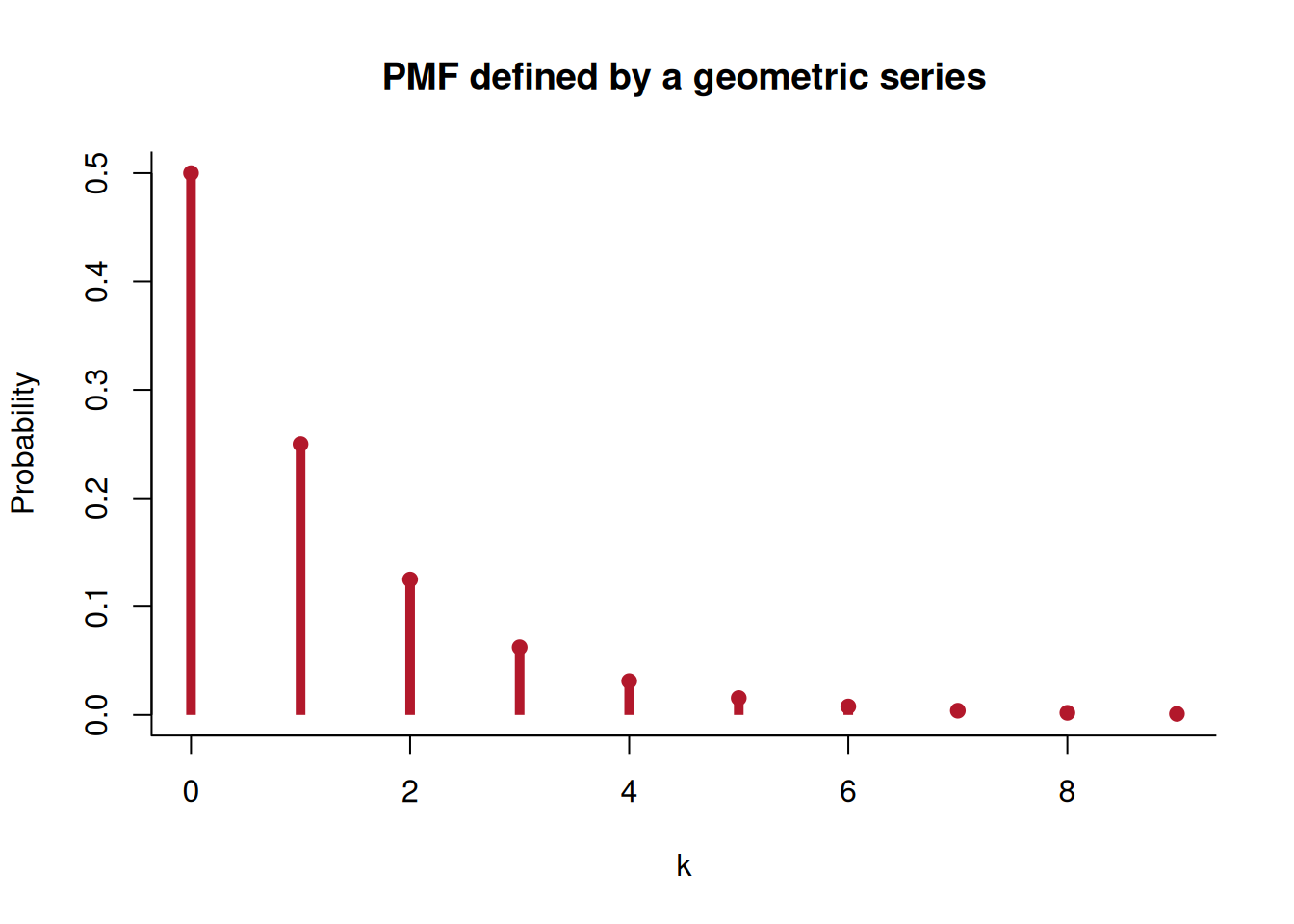
Suppose we sample word tokens until the first loanword appears. The response is not a fixed number of trials. It is the number of nonloanwords we see before the target. What distribution represents this waiting count?
This is a methodological example. A corpus application would need an explicit operational definition of loanword and a token-sampling order; the geometric model does not decide disputed etymological or borrowing classifications.
To begin with a particular case, suppose the loanword probability is 1/2 on each independent draw. Zero failures occurs with probability 1/2, one failure followed by a target with probability 1/4, and two failures followed by a target with probability 1/8. These probabilities form the geometric series
\sum_{k=0}^{\infty}\frac{1}{2^{k+1}}=1.
Thus p_K(k)\equiv2^{-(k+1)}, for k=0,1,2,\ldots, is a probability mass function (PMF) with countably infinite support. The index k counts failures, so the first term corresponds to an immediate target.
k <- 0:9
mass <- 2^(-(k + 1))
plot(k, mass, type = "h", lwd = 5, lend = 1, col = "#B2182B",
xlab = "k", ylab = "Probability",
main = "PMF defined by a geometric series", bty = "l")
points(k, mass, pch = 19, col = "#B2182B")
Basically, the geometric distribution extends this example from target probability 1/2 to any fixed target probability. More specifically, the geometric distribution models a waiting count. Let K count failures before the first success in independent Bernoulli trials with common success probability \pi\in(0,1]. We define
K\sim\operatorname{Geometric}(\pi)
by
p_K(k) \equiv\mathbb P(K=k) =(1-\pi)^k\pi, \qquad k=0,1,2,\ldots.
This is the convention used by dgeom in R. If T counts total trials through the first success, then T\equiv K+1 and
\mathbb P(T=t)=(1-\pi)^{t-1}\pi, \qquad t=1,2,\ldots.
Suppose we sample word tokens until the first loanword, with constant loanword probability \pi=.20. The event K=k requires k nonloanwords followed by one loanword. Independence gives
\mathbb P(K=k)=(.80)^k(.20).
Thus
\begin{aligned} p_K(0)&=.20,\\ p_K(1)&=.80(.20)=.16,\\ p_K(2)&=.80^2(.20)=.128,\\ p_K(3)&=.80^3(.20)=.1024. \end{aligned}
The event K\geq4 requires four initial failures, so
\mathbb P(K\geq4)=.80^4=.4096
and \mathbb P(T\leq4)=1-.4096=.5904.
The following graphs compare \pi=.5, .1, and .9.
plot_geometric <- function(probability) {
  k <- 0:9
  mass <- dgeom(k, prob = probability)
  plot(k, mass, type = "h", lwd = 5, lend = 1, col = "#B2182B",
       xlab = "Failures before the first success", ylab = "Probability",
       main = sprintf("PMF of Geometric(%.1f)", probability), bty = "l")
  points(k, mass, pch = 19, col = "#B2182B")
}

plot_geometric(.5)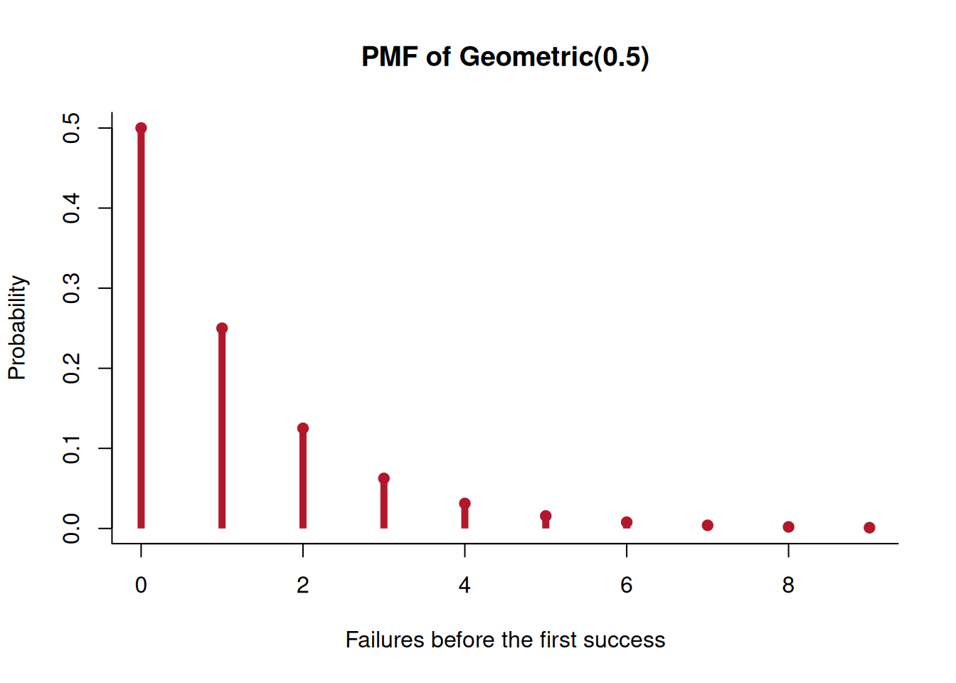
plot_geometric(.1)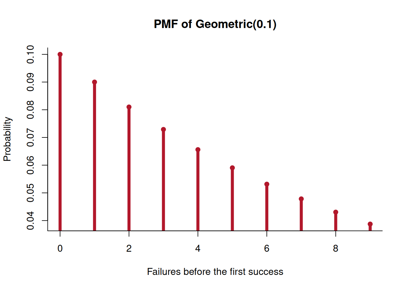
plot_geometric(.9)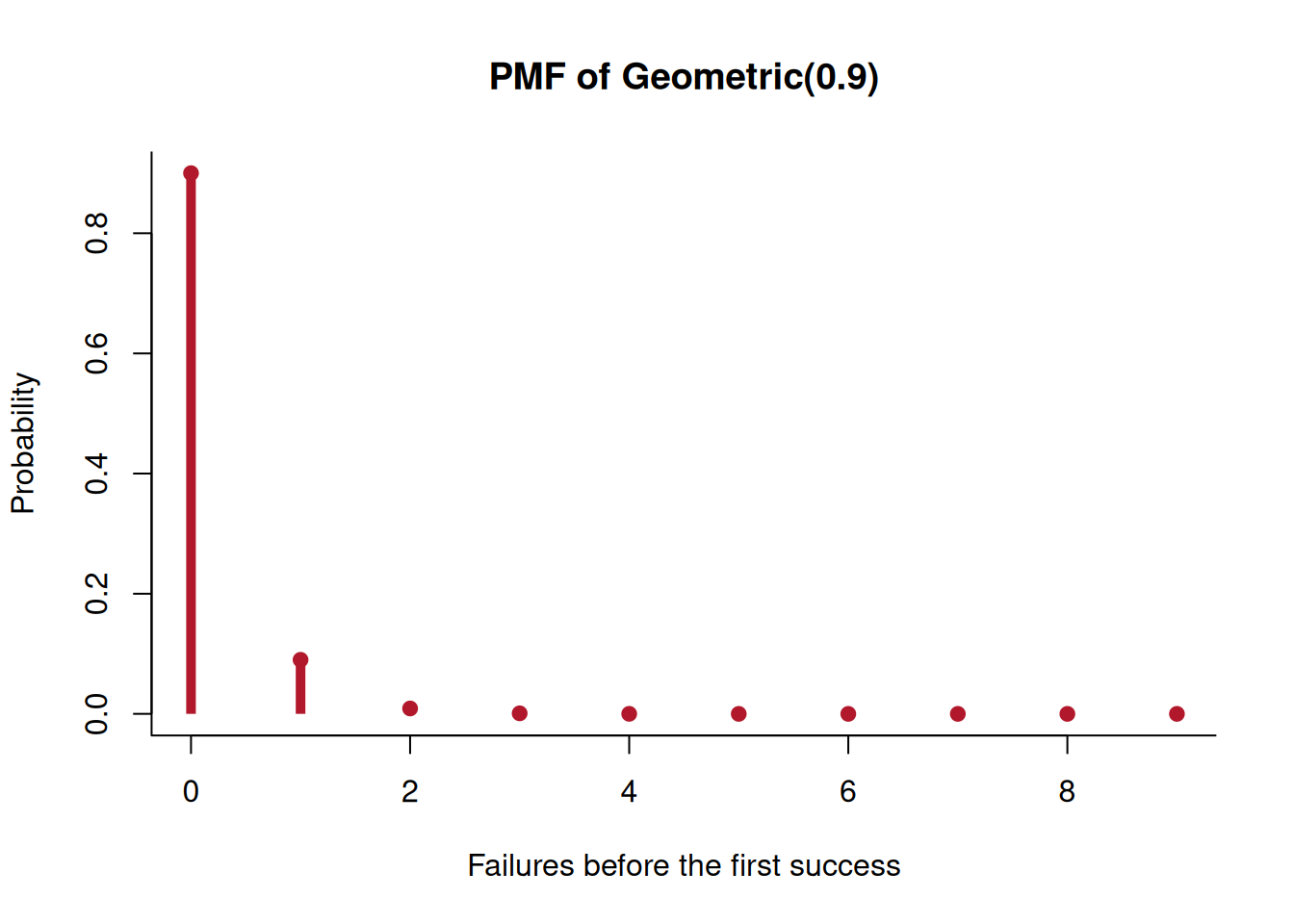
For every k\geq0,
\frac{p_K(k+1)}{p_K(k)} =1-\pi<1.
Thus every nondegenerate geometric PMF is strictly decreasing. Its mode is K=0. If L\equiv K+1 represents positive word length, its mode is necessarily L=1. The negative-binomial page compares this restriction with the empirical distribution of phoneme counts in CMUdict.
Let q\equiv1-\pi. Differentiating the geometric series gives
\sum_{k=0}^{\infty}q^k=\frac{1}{1-q} \quad\Longrightarrow\quad \sum_{k=1}^{\infty}kq^{k-1}=\frac{1}{(1-q)^2}.
Thus
\begin{aligned} \mathbb E[K] &=\sum_{k=0}^{\infty}kq^k\pi\\ &=\pi q\sum_{k=1}^{\infty}kq^{k-1}\\ &=\frac{1-\pi}{\pi}. \end{aligned}
Differentiating the geometric series twice also gives
\mathbb E[K(K-1)] =\frac{2(1-\pi)^2}{\pi^2}.
Since K^2=K(K-1)+K,
\begin{aligned} \operatorname{Var}(K) &=\mathbb E[K^2]-\mathbb E[K]^2\\ &=\mathbb E[K(K-1)]+\mathbb E[K]-\mathbb E[K]^2\\ &=\frac{1-\pi}{\pi^2}. \end{aligned}
The algebra matches the waiting-time interpretation. A smaller target probability increases both the expected number of failures and the uncertainty about how long the wait will be.
The geometric family waits for one target. The negative-binomial page keeps the same trial assumptions but waits for a declared number of targets.