---
title: "The beta distribution"
execute:
enabled: true
echo: true
warning: false
message: false
---
The [uniform distribution](uniform-distribution.qmd) placed constant density on a bounded interval. But suppose values near $.2$ should receive more density than values near $.8$, even though both lie in the unit interval. How can we change the shape while keeping the same bounds? Let $\Theta$ represent a speaker's latent probability of choosing the double object construction in a declared discourse context.
The substantive question is how construction choice varies across comparable dative tokens and contexts, a distinction studied in corpus work on the [English dative alternation](https://web.stanford.edu/~bresnan/qs-submit.pdf). The latent probability is a model quantity. It is not one observed token choice, and its variation does not by itself explain the alternation.
The [**beta distribution**](https://bruno.nicenboim.me/bayescogsci/ch-introBDA.html) is a family of absolutely continuous distributions with topological support $[0,1]$:
$$
\Theta\sim\operatorname{Beta}(\alpha,\beta),
\qquad \alpha>0,\ \beta>0.
$$
Its density has the form
$$
f_\Theta(\theta)
\equiv
\begin{cases}
\dfrac{\theta^{\alpha-1}(1-\theta)^{\beta-1}}
{B(\alpha,\beta)},&0<\theta<1,\\
0,&\text{otherwise}.
\end{cases}
$$
The normalizing constant is the beta function
$$
B(\alpha,\beta)
\equiv
\int_0^1 t^{\alpha-1}(1-t)^{\beta-1}\,\mathrm dt.
$$
The beta function in the denominator is the normalizing constant: it is exactly the integral of the numerator over $(0,1)$. Dividing by it makes the total density area one. The parameters $\alpha$ and $\beta$ control how that unit probability mass is arranged across the interval.
## Beginning from constant density
Set $\alpha=1$ and $\beta=1$. Then
$$
\theta^{\alpha-1}(1-\theta)^{\beta-1}
=\theta^0(1-\theta)^0
=1.
$$
The density is constant across $(0,1)$. This case matches a uniform density on the unit interval.
## Changing the relative parameter sizes
When $\alpha>\beta$, more density tends to lie toward one. When $\beta>\alpha$, more density tends to lie toward zero.
For instance, $\operatorname{Beta}(5,2)$ places more density on high construction preference values, while $\operatorname{Beta}(2,5)$ places more on low values. Interchanging the parameters reflects the density around $.5$.
When both parameters exceed one, the density may have an interior peak. When both lie below one, density may rise near both boundaries. The family can thus represent several shapes with the same bounded support.
## Deriving the mean and variance
By the definition of expectation,
$$
\begin{aligned}
\mathbb E[\Theta]
&=\frac{1}{B(\alpha,\beta)}
\int_0^1\theta^\alpha(1-\theta)^{\beta-1}\,\mathrm d\theta\\
&=\frac{B(\alpha+1,\beta)}{B(\alpha,\beta)}\\
&=\frac{\alpha}{\alpha+\beta}.
\end{aligned}
$$
The first equality inserts the beta density into the expectation integral. Multiplying by $\theta$ raises its exponent from $\alpha-1$ to $\alpha$, so the resulting integral is $B(\alpha+1,\beta)$. The final step uses the beta-function recurrence
$$
B(\alpha+1,\beta)
=\frac{\alpha}{\alpha+\beta}B(\alpha,\beta).
$$
Each equality thus follows from either the expectation definition or the beta-function identity.
For $\operatorname{Beta}(2,5)$,
$$
\mathbb{E}[\Theta]
=\frac{2}{7}
\approx.286.
$$
Similarly,
$$
\mathbb E[\Theta^2]
=\frac{B(\alpha+2,\beta)}{B(\alpha,\beta)}
=\frac{\alpha(\alpha+1)}{(\alpha+\beta)(\alpha+\beta+1)}.
$$
Thus
$$
\begin{aligned}
\operatorname{Var}(\Theta)
&=\mathbb E[\Theta^2]-\mathbb E[\Theta]^2\\
&=\frac{\alpha\beta}
{ (\alpha+\beta)^2(\alpha+\beta+1)}.
\end{aligned}
$$
For $\operatorname{Beta}(2,5)$,
$$
\operatorname{Var}(\Theta)
=\frac{10}{49(8)}
\approx.0255.
$$
The parameters jointly determine center and concentration. Neither parameter alone is a mean or variance.
## Holding the mean fixed while changing concentration
If $\Theta_1\sim\operatorname{Beta}(2,2)$ and $\Theta_2\sim\operatorname{Beta}(20,20)$, both variables have mean $.5$, but
$$
\operatorname{Var}(\Theta_1)=.05
$$
and
$$
\operatorname{Var}(\Theta_2)\approx.0061.
$$
The larger equal parameters concentrate more density near $.5$. Equal means do not imply equal variances.
## Inspecting the shapes in base R
```{r}
#| eval: false
theta <- seq(.001, .999, length.out = 300)

plot(theta, dbeta(theta, 2, 5), type = "l",
     xlab = "double object preference", ylab = "density")
lines(theta, dbeta(theta, 5, 2), lty = 2)
lines(theta, dbeta(theta, 2, 2), lty = 3)
lines(theta, dbeta(theta, 20, 20), lty = 4)
```
The plot separates changes in location from changes in concentration.
## Keeping the modeled level explicit
The variable $\Theta$ is a latent probability for a speaker and context. It is not one binary construction choice. A single token remains a zero and one outcome, while $\Theta$ describes the chance of the target outcome across comparable tokens.
A proportion calculated from finitely many observed tokens is also not automatically a direct beta observation. Its discreteness and denominator remain part of the measurement process.
## Checking the response support
A beta distribution is not appropriate merely because a response is written between zero and one. The family is continuous on the open interval and assigns no probability to exact endpoints. A response process that produces structural zeros, structural ones, or a finite grid needs those features represented explicitly.
Support is necessary but not sufficient. The modeled level and observation process must also match.
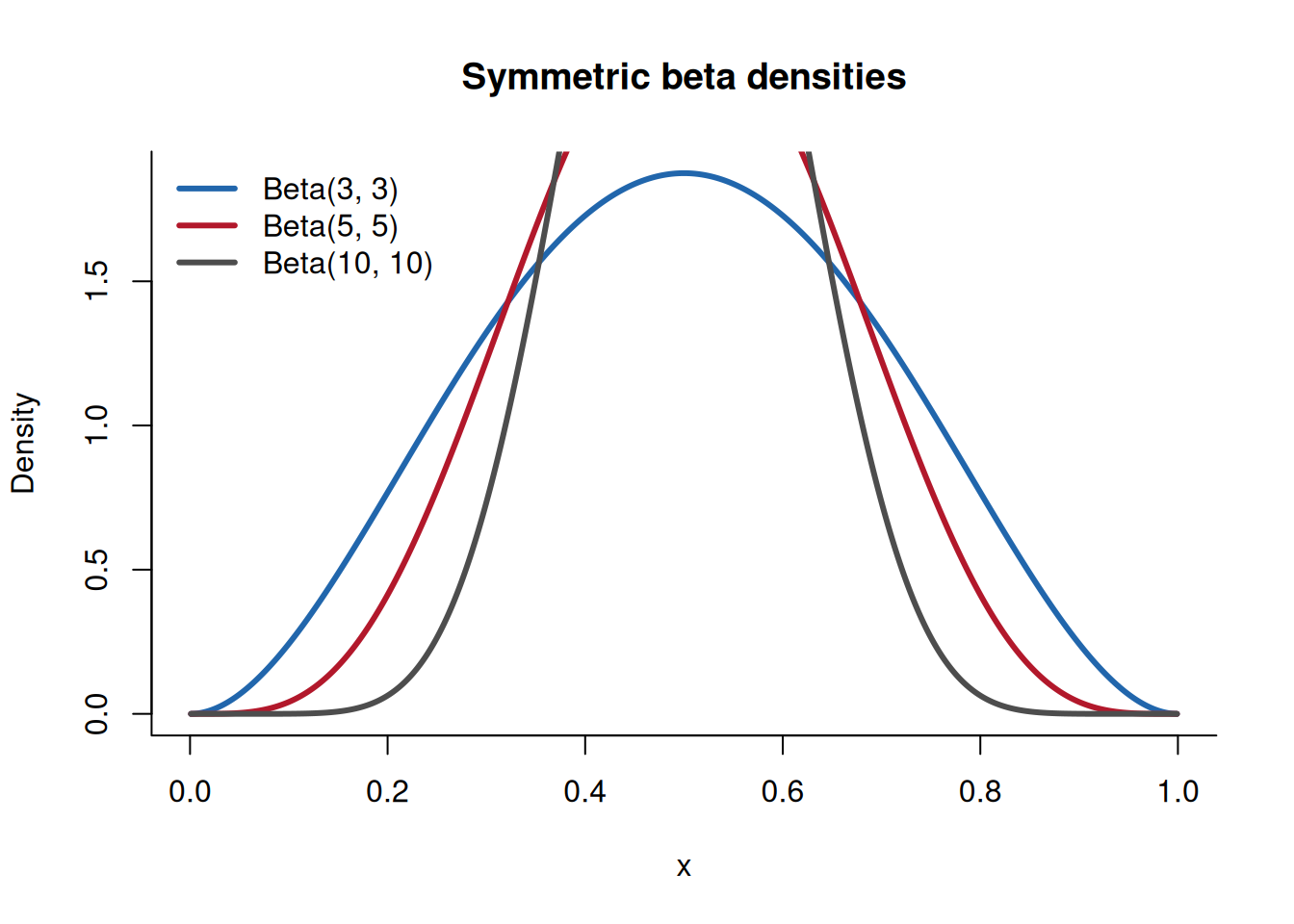
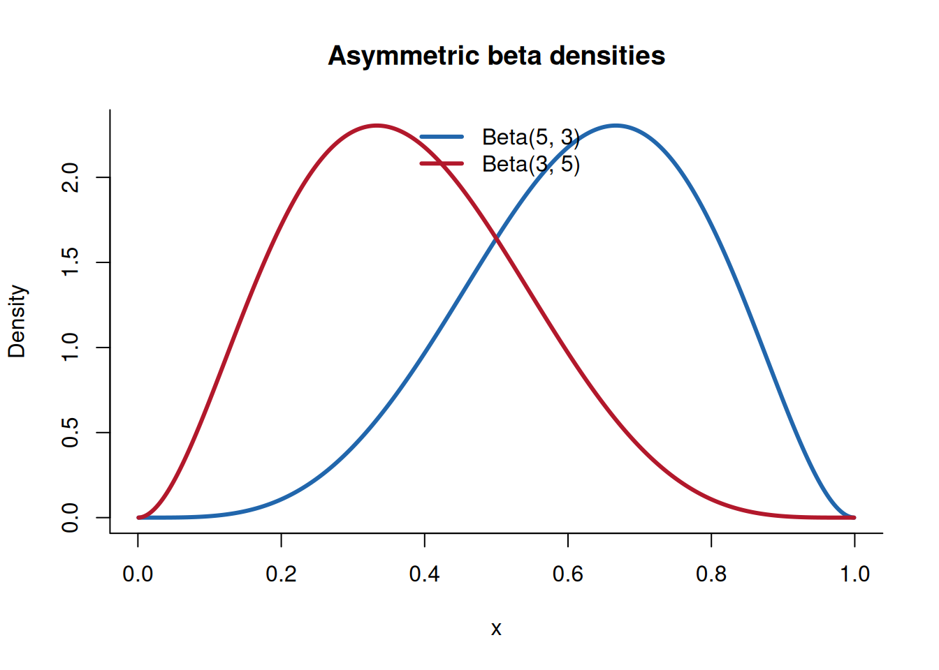
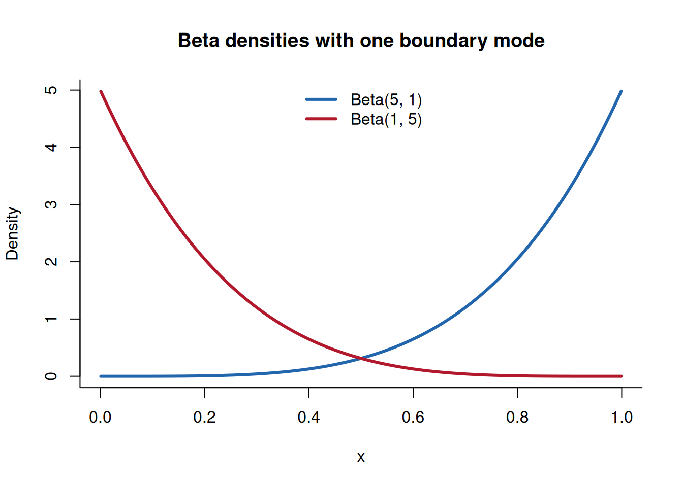
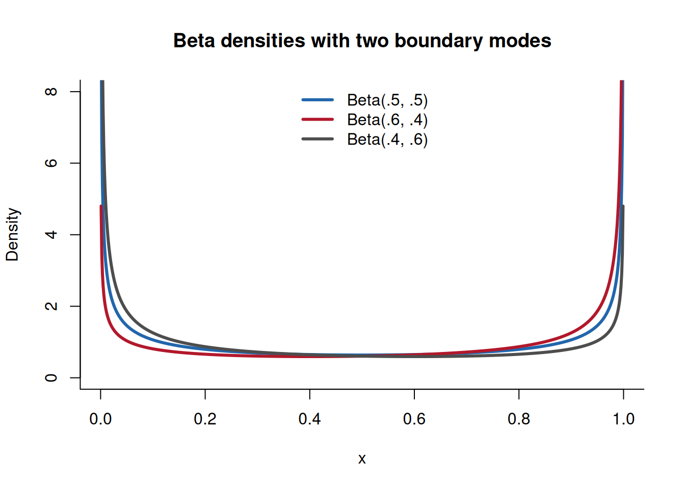
## A sequence of beta shapes
First, equal parameters greater than one produce symmetric densities with an interior mode.
```{r}
x_beta <- seq(.001, .999, length.out = 800)
plot(x_beta, dbeta(x_beta, 3, 3), type = "l", lwd = 3,
     col = "#2166AC", xlab = "x", ylab = "Density",
     main = "Symmetric beta densities", bty = "l")
lines(x_beta, dbeta(x_beta, 5, 5), lwd = 3, col = "#B2182B")
lines(x_beta, dbeta(x_beta, 10, 10), lwd = 3, col = "#4D4D4D")
legend("topleft", c("Beta(3, 3)", "Beta(5, 5)", "Beta(10, 10)"),
       col = c("#2166AC", "#B2182B", "#4D4D4D"),
       lty = 1, lwd = 3, bty = "n")
```
Second, unequal parameters greater than one move the interior mode away from $.5$.
```{r}
plot(x_beta, dbeta(x_beta, 5, 3), type = "l", lwd = 3,
     col = "#2166AC", xlab = "x", ylab = "Density",
     main = "Asymmetric beta densities", bty = "l")
lines(x_beta, dbeta(x_beta, 3, 5), lwd = 3, col = "#B2182B")
legend("top", c("Beta(5, 3)", "Beta(3, 5)"),
       col = c("#2166AC", "#B2182B"), lty = 1, lwd = 3, bty = "n")
```
Third, setting one parameter to one and the other above one produces a single boundary mode.
```{r}
plot(x_beta, dbeta(x_beta, 5, 1), type = "l", lwd = 3,
     col = "#2166AC", xlab = "x", ylab = "Density",
     main = "Beta densities with one boundary mode", bty = "l")
lines(x_beta, dbeta(x_beta, 1, 5), lwd = 3, col = "#B2182B")
legend("top", c("Beta(5, 1)", "Beta(1, 5)"),
       col = c("#2166AC", "#B2182B"), lty = 1, lwd = 3, bty = "n")
```
Fourth, $\alpha<1$ and $\beta<1$ produce two boundary modes.
```{r}
plot(x_beta, dbeta(x_beta, .5, .5), type = "l", lwd = 3,
     col = "#2166AC", xlab = "x", ylab = "Density",
     main = "Beta densities with two boundary modes",
     ylim = c(0, 8), bty = "l")
lines(x_beta, dbeta(x_beta, .6, .4), lwd = 3, col = "#B2182B")
lines(x_beta, dbeta(x_beta, .4, .6), lwd = 3, col = "#4D4D4D")
legend("top", c("Beta(.5, .5)", "Beta(.6, .4)", "Beta(.4, .6)"),
       col = c("#2166AC", "#B2182B", "#4D4D4D"),
       lty = 1, lwd = 3, bty = "n")
```
These graphs show which features each parameter change controls.
## Transforming the support to an arbitrary finite interval
Let $X\sim\operatorname{Beta}(\alpha,\beta)$ and define
$$
Y\equiv a+(b-a)X,
\qquad a<b.
$$
Then $Y$ has density
$$
f_Y(y)
\equiv
\begin{cases}
\dfrac{1}{b-a}
\dfrac{
\left(\frac{y-a}{b-a}\right)^{\alpha-1}
\left(1-\frac{y-a}{b-a}\right)^{\beta-1}
}{B(\alpha,\beta)},&a<y<b,\\[4mm]
0,&\text{otherwise}.
\end{cases}
$$
The factor $1/(b-a)$ is the Jacobian of the linear transformation and is required for the density to integrate to one.
## Check your understanding
1. Compute the mean of $\operatorname{Beta}(3,7)$.
2. Why do $\operatorname{Beta}(2,2)$ and $\operatorname{Beta}(20,20)$ have the same mean but different concentration?
3. Explain the difference between a latent construction probability and one observed construction choice.
4. Why can exact endpoint responses cause a support mismatch for a direct beta model?
The beta family changes shape within a bounded interval. The [next page](normal-distribution.qmd) introduces a symmetric location and scale family over the full real line.