---
title: $N$-gram models
bibliography: ../references.bib
jupyter: python3
---
In the previous section, I defined a language model as a specification of a probability measure on $\Sigma^*$ and showed that the chain rule gives us an exact decomposition:
$$p(w_1 w_2 \ldots w_n) = p(w_1) \prod_{i=2}^{n} p(w_i \mid w_1 \ldots w_{i-1})$$
The trouble with using this decomposition directly is that each conditional $p(w_i \mid w_1 \ldots w_{i-1})$ depends on the entire prefix $w_1 \ldots w_{i-1}$. As the prefix gets longer, the number of possible prefixes grows exponentially: there are $|\Sigma|^{i-1}$ possible prefixes of length $i - 1$. Estimating a separate distribution for every possible prefix would require an enormous amount of data and memory, and for most prefixes we'd never observe enough examples to get a reliable estimate.
An $N$-gram model deals with this by making an independence assumption: the distribution of $w_i$ depends only on the preceding $N - 1$ symbols, not on the entire prefix. That is:
$$p(w_i \mid w_1 \ldots w_{i-1}) \approx p(w_i \mid w_{i-N+1} \ldots w_{i-1})$$
Substituting this approximation into the exact chain rule decomposition gives us:
$$p(w_1 w_2 \ldots w_n) \approx \prod_{i=1}^{n+1} p(w_i \mid w_{i-N+1} \ldots w_{i-1})$$
where we pad the beginning of the string with $N-1$ copies of a start symbol $\langle\text{s}\rangle$ and append an end symbol $\langle\text{/s}\rangle$ at position $n + 1$.^[The start and end symbols ensure that the model can learn which phones tend to begin and end words. Without them, the model wouldn't distinguish between a phone that appears word-initially and one that appears word-medially.]
Each conditional distribution $p(w_i \mid w_{i-N+1} \ldots w_{i-1})$ is a categorical distribution over $\Sigma$ (plus the end symbol), parameterized by a vector $\boldsymbol{\theta}^{(w_{i-N+1} \ldots w_{i-1})}$. So the full model is parameterized by a collection $\boldsymbol{\Theta}$ of such vectors—one for each possible context of length $N - 1$.
## Maximum likelihood estimation
Given a corpus of strings, we want to find the parameters $\boldsymbol{\Theta}$ that maximize the likelihood of the observed data. For a unigram model ($N = 1$), where there is no conditioning context, this amounts to:
$$\hat{\boldsymbol{\Theta}}_\text{MLE} = \arg_{\boldsymbol{\Theta}}\max \prod_{j=1}^{V} \theta_j^{c_j}$$
where $c_j$ is the number of times phone $j$ occurs in the corpus and $V = |\Sigma|$. The solution is to set each $\theta_j$ proportional to its count:
$$\hat{\theta}_j = \frac{c_j}{\sum_k c_k}$$
More generally, for any $N$-gram model:
$$\hat{\theta}_{w_{i_1} \ldots w_{i_N}} = \frac{c_{i_1 i_2 \ldots i_N}}{\sum_j c_{i_1 i_2 \ldots j}}$$
where $c_{i_1 i_2 \ldots i_N}$ is the number of times the sequence $w_{i_1} \ldots w_{i_N}$ occurs in the corpus. In words: the estimated probability of a phone given a context is just the proportion of times that phone follows that context in the training data.
## Smoothing
One issue with the MLE is that any $N$-gram that never occurs in the training data will be assigned probability zero. This is a problem because when we compute the probability of a string, we multiply conditionals together—and a single zero sends the entire product to zero. In log space, this looks like a single $-\infty$ sending the sum to $-\infty$.
To see why this matters concretely, consider a bigram model trained on a typical English lexicon. The sequence $\text{ŋk}$ probably appears many times (as in *think*, *bank*), so the model learns a reasonable estimate of $p(\text{k} \mid \text{ŋ})$. But the sequence $\text{ŋm}$ may never appear in the training data at all, so the MLE assigns $p(\text{m} \mid \text{ŋ}) = 0$. Now suppose we want to evaluate a nonword that happens to contain $\text{ŋm}$. Under the MLE, the entire string gets probability zero—not because it's maximally bad, but because the model has never seen that one transition. A single gap in the training data wipes out all the information from the other transitions in the string.
### Add-$\lambda$ smoothing
The fix is to ensure that no $N$-gram probability is ever exactly zero. [Add-$\lambda$ smoothing](https://en.wikipedia.org/wiki/Additive_smoothing) (also called Laplace smoothing when $\lambda = 1$) does this by adding a pseudocount $\lambda > 0$ to every $N$-gram count before normalizing:
$$\hat{\theta}_{w_{i_1} \ldots w_{i_N}} = \frac{c_{i_1 i_2 \ldots i_N} + \lambda}{\sum_j \left[c_{i_1 i_2 \ldots j} + \lambda\right]}$$
The pseudocount works as if we had observed each possible $N$-gram $\lambda$ additional times on top of whatever the data actually contains. This has two effects. First, no probability is ever zero: even an $N$-gram that never occurred in the training data gets a small positive probability proportional to $\lambda$. Second, the probabilities of frequently observed $N$-grams are slightly reduced to make room, since the denominator grows by $|\Sigma| \cdot \lambda$ (the total pseudocounts across all phones that could follow the context).
The parameter $\lambda$ controls the strength of this effect, and it is worth understanding its two extremes:
- When $\lambda = 0$, we recover the MLE exactly. The model trusts the data completely: observed counts determine probabilities, and unseen $N$-grams get probability zero.
- As $\lambda \to \infty$, the pseudocounts overwhelm the observed counts and every conditional distribution converges to uniform: $\hat{\theta} \to 1/|\Sigma|$ for all contexts. The model ignores the data entirely and assigns equal probability to all phones in all positions.
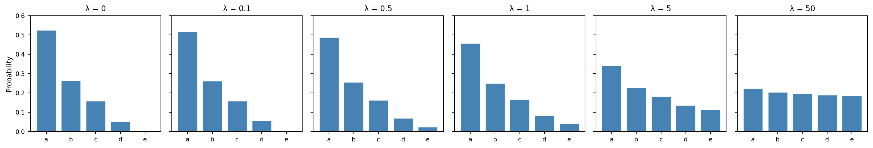
Between these extremes, $\lambda$ interpolates between fitting the data closely and hedging toward a uniform distribution. The following plot illustrates this on a toy example: a unigram distribution over 5 phones with counts $(10, 5, 3, 1, 0)$. As $\lambda$ increases, the distribution flattens from the MLE toward uniform.
```{python}
#| code-fold: true
#| code-summary: Effect of smoothing on a toy distribution
import numpy as np
import matplotlib.pyplot as plt

counts = np.array([10, 5, 3, 1, 0])
phones = ['a', 'b', 'c', 'd', 'e']
lambdas = [0, 0.1, 0.5, 1, 5, 50]

fig, axes = plt.subplots(1, len(lambdas), figsize=(16, 2.8), sharey=True)

for ax, lam in zip(axes, lambdas):
    smoothed = (counts + lam) / (counts.sum() + lam * len(counts))
    ax.bar(phones, smoothed, color='steelblue', edgecolor='white')
    ax.set_title(f'λ = {lam}', fontsize=10)
    ax.set_ylim(0, 0.6)
    ax.tick_params(labelsize=8)
    if lam == 0:
        ax.set_ylabel('Probability', fontsize=9)

fig.tight_layout()
plt.show()
```
A small $\lambda$ stays close to the observed frequencies while giving unseen $N$-grams just enough probability to avoid zeros. A large $\lambda$ washes out the distinctions the model learned from the data. The right value of $\lambda$ depends on how much data we have and how much we trust the model's specific estimates—which is exactly the kind of question that [cross-validation](#evaluating-a-predictor) can answer.^[For those interested: add-$\lambda$ smoothing corresponds to placing a symmetric [Dirichlet prior](https://en.wikipedia.org/wiki/Dirichlet_distribution) $\text{Dir}(\boldsymbol{1} + \lambda)$ on each conditional distribution and computing a [maximum a posteriori](https://en.wikipedia.org/wiki/Maximum_a_posteriori_estimation) (MAP) estimate rather than an MLE. The pseudocounts are the prior's way of encoding a belief about what the distribution looks like before seeing any data. When $\lambda = 0$—a uniform Dirichlet $\text{Dir}(\boldsymbol{1})$—the MAP estimate reduces to the MLE. See @hastie_elements_2009[Ch. 8] for a broader discussion of regularization, of which smoothing is a special case.]
Add-$\lambda$ smoothing is the simplest member of a large family of smoothing techniques for $N$-gram models, all of which address the same core problem—redistributing probability mass from observed $N$-grams to unobserved ones—but differ in how they decide how much mass to redistribute and where to put it. [Good-Turing smoothing](https://en.wikipedia.org/wiki/Good%E2%80%93Turing_frequency_estimation) [@good_population_1953] estimates the total probability of unseen events from the number of events seen exactly once. [Jelinek-Mercer smoothing](https://en.wikipedia.org/wiki/Jelinek%E2%80%93Mercer_smoothing) [@jelinek_interpolated_1980] interpolates between higher-order and lower-order $N$-gram estimates, so that a trigram model can fall back to a bigram estimate when the trigram count is sparse. [Katz backoff](https://en.wikipedia.org/wiki/Katz%27s_back-off_model) [@katz_estimation_1987] takes a similar approach but uses the lower-order model only when the higher-order count falls below a threshold. [Kneser-Ney smoothing](https://en.wikipedia.org/wiki/Kneser%E2%80%93Ney_smoothing) [@kneser_improved_1995] refines this further by basing the lower-order distribution not on raw counts but on the number of distinct contexts in which a word appears, which gives better estimates for words that are common only in a few fixed phrases. @chen_empirical_1996 provide a thorough empirical comparison of these methods. We use add-$\lambda$ smoothing here because it is easy to implement and sufficient for our purposes, but the more sophisticated methods are standard in large-scale language modeling.
We can thus view an $N$-gram model as having two hyperparameters: the order $N$, which determines how much context the model conditions on, and the smoothing parameter $\lambda$, which determines how much it trusts the observed counts versus a uniform fallback.
## Fitting $N$-gram models to a lexicon
To see how well $N$-gram models predict phonotactic acceptability, we'll fit models to the [CMU Pronouncing Dictionary](https://web.archive.org/web/20210216211828/http://www.speech.cs.cmu.edu/cgi-bin/cmudict) and evaluate them against the acceptability judgments from @daland_explaining_2011.
We begin by loading the dictionary, which uses the [ARPABET](https://en.wikipedia.org/wiki/ARPABET) representation, and converting it to IPA.
```{python}
#| code-fold: true
#| code-summary: Load CMU Pronouncing Dictionary and convert to IPA
import re
import numpy as np
import pandas as pd
import nltk

nltk.download('cmudict', quiet=True)

from nltk.corpus import cmudict

arpabet_to_phoneme = {
    'AA': 'ɑ', 'AE': 'æ', 'AH': 'ʌ', 'AO': 'ɔ', 'AW': 'aʊ', 'AY': 'aɪ',
    'B': 'b', 'CH': 'tʃ', 'D': 'd', 'DH': 'ð', 'EH': 'ɛ', 'ER': 'ɝ',
    'EY': 'eɪ', 'F': 'f', 'G': 'g', 'HH': 'h', 'IH': 'ɪ', 'IY': 'i',
    'JH': 'dʒ', 'K': 'k', 'L': 'l', 'M': 'm', 'N': 'n', 'NG': 'ŋ',
    'OW': 'oʊ', 'OY': 'ɔɪ', 'P': 'p', 'R': 'ɹ', 'S': 's', 'SH': 'ʃ',
    'T': 't', 'TH': 'θ', 'UH': 'ʊ', 'UW': 'u', 'V': 'v', 'W': 'w',
    'Y': 'j', 'Z': 'z', 'ZH': 'ʒ'
}

entries = {
    word: [arpabet_to_phoneme[re.sub(r'[0-9]', '', phone)] for phone in phones]
    for word, phones in cmudict.entries()
    if len(set(word)) > 1
    if len(phones) > 1
    if not re.findall(r'[^a-z]', word)
}

len(entries)
```
Next, we define the $N$-gram model. The implementation stores log-probabilities to avoid numerical underflow.
```{python}
#| code-fold: true
#| code-summary: Define `NgramModel`
from collections.abc import Iterable
from collections import defaultdict, Counter
from itertools import product

alphabet = {phone for phones in entries.values() for phone in phones}


class NgramModel:
    """An N-gram language model with add-lambda smoothing.

    Parameters
    ----------
    alphabet : set[str]
        The set of symbols in the language.
    n : int
        The order of the model (default 2 for bigram).
    lam : float
        The smoothing pseudocount (default 0 for MLE).
    """

    def __init__(self, alphabet: set[str], n: int = 2, lam: float = 0.):
        self._alphabet = alphabet
        self._n = n
        self._lam = lam

    def predict(self, string: list[str]) -> float:
        """Compute the log-probability of a string.

        Parameters
        ----------
        string : list[str]
            The phone sequence to score.

        Returns
        -------
        float
            The log-probability of the string under the model.
        """
        padded = ['<s>'] * (self._n - 1) + list(string) + ['</s>']

        logprob = 0.
        for i in range(self._n - 1, len(padded)):
            context = tuple(padded[i - self._n + 1:i])
            token = padded[i]

            if self._n == 1:
                context = ()
                if token in ('<s>',):
                    continue

            if context in self._logprob and token in self._logprob[context]:
                logprob += self._logprob[context][token]
            else:
                logprob += -np.inf

        return logprob

    def fit(self, lexicon: Iterable[list[str]]) -> 'NgramModel':
        """Fit the model to a lexicon of phone sequences.

        Parameters
        ----------
        lexicon : Iterable[list[str]]
            An iterable of phone sequences to train on.

        Returns
        -------
        NgramModel
            The fitted model (self).
        """
        vocab = self._alphabet | {'</s>'}

        freq: dict[tuple, Counter] = {}

        # Contexts that start with <s> padding
        for k in range(1, self._n):
            for ctx in product(*[self._alphabet] * (k - 1)):
                full_ctx = tuple(['<s>'] * (self._n - k)) + ctx
                freq[full_ctx] = Counter({v: 0 for v in vocab})

        # All other contexts
        for ctx in product(*[self._alphabet] * (self._n - 1)):
            freq[ctx] = Counter({v: 0 for v in vocab})

        # Unigram context
        if self._n == 1:
            freq[()] = Counter({v: 0 for v in vocab})

        # Count N-grams
        for word in lexicon:
            padded = ['<s>'] * (self._n - 1) + list(word) + ['</s>']
            for i in range(self._n - 1, len(padded)):
                context = tuple(padded[i - self._n + 1:i])
                token = padded[i]
                if self._n == 1:
                    context = ()
                    if token == '<s>':
                        continue
                if context in freq:
                    freq[context][token] += 1

        # Compute log-probabilities with add-λ smoothing
        self._logprob = {
            ctx: {
                tok: np.log(count + self._lam) -
                     np.log(sum(counts.values()) + len(counts) * self._lam)
                for tok, count in counts.items()
            }
            for ctx, counts in freq.items()
        }

        return self
```
We'll fit models with $N \in \{1, 2, 3, 4\}$ and a range of smoothing values $\lambda \in \{0, 0.1, 0.5, 1, 2, 5, 10\}$.
```{python}
models = defaultdict(dict)

for n in range(1, 5):
    for lam in [0., 0.1, 0.5, 1., 2., 5., 10.]:
        models[n][lam] = NgramModel(alphabet, n=n, lam=lam).fit(entries.values())
```
## A few test cases
To get an initial sense for how these models behave, we can look at the probabilities they assign to a few test words. These are constructed to have the same vowel and coda but different onsets, ranging from well-attested ($\text{blɪk}$) to unattested ($\text{bnɪk}$, $\text{bzɪk}$, $\text{bsɪk}$).
```{python}
test_words = [
    ['b', 'l', 'ɪ', 'k'],
    ['b', 'n', 'ɪ', 'k'],
    ['b', 'z', 'ɪ', 'k'],
    ['b', 's', 'ɪ', 'k'],
]

for n in [2, 3]:
    for lam in [0., 1.]:
        print(f'N={n}, λ={lam}:')
        for w in test_words:
            print(f'  {"".join(w):6s} {models[n][lam].predict(w):8.2f}')
        print()
```
Notice that the models with $N > 1$ consistently assign higher probability to $\text{blɪk}$ (which has an attested onset cluster) than to $\text{bnɪk}$, $\text{bzɪk}$, or $\text{bsɪk}$ (which do not). The unigram model doesn't make this distinction, since it doesn't condition on previous phones at all.
## Predicting acceptability
Now let's ask a more systematic question: how well do these models predict the acceptability judgments from @daland_explaining_2011? We load the acceptability data and convert the ARPABET representations to IPA.
```{python}
#| code-fold: true
#| code-summary: Load acceptability data and convert to IPA
acceptability = pd.read_csv('Daland_etal_2011__AverageScores.csv')
acceptability['phono_cmu'] = acceptability.phono_cmu.str.strip('Coda').str.split()


def map_to_ipa(phones: list[str]) -> list[str]:
    """Convert ARPABET phone list to IPA symbols.

    Parameters
    ----------
    phones : list[str]
        ARPABET phone symbols, possibly with stress digits.

    Returns
    -------
    list[str]
        The corresponding IPA symbols.
    """
    return [arpabet_to_phoneme[re.sub(r'[0-9]', '', p)] for p in phones]


acceptability['phono_ipa'] = acceptability.phono_cmu.map(map_to_ipa)
```
The approach is straightforward. For each model, we compute the log-probability of each nonword in the dataset, then ask how well that log-probability predicts the human acceptability rating. We test the hypothesis that the relationship is linear:
$$a_\mathbf{w} \sim \mathcal{N}(m \log p(\mathbf{w} \mid \boldsymbol\Theta) + b, \sigma^2)$$
Because all the nonwords in the dataset happen to be the same length, we don't need to worry about length normalization here—though in general, we would need to, since longer strings tend to have lower log-probabilities simply because more terms are being multiplied together.
### Evaluating a predictor
Before we run the evaluation, it's worth spelling out the machinery we'll use, since the same ideas will recur throughout these notes.
#### Linear regression
The model above says that a nonword's acceptability rating is, in expectation, a linear function of its log-probability. We defined [conditional expectation](some-more-useful-definitions.qmd#conditional-expectation) earlier as $\mathbb{E}[X \mid Y = y] = \sum_x x \cdot p(x \mid y)$; the claim here is that $\mathbb{E}[a_\mathbf{w} \mid \log p(\mathbf{w} \mid \boldsymbol\Theta) = x] = mx + b$ for some slope $m$ and intercept $b$. The Gaussian noise term $\sigma^2$ captures everything about the rating that the log-probability doesn't predict.
To *fit* this model—to find $m$ and $b$—we use [ordinary least squares](https://en.wikipedia.org/wiki/Ordinary_least_squares): choose the values of $m$ and $b$ that minimize the sum of squared residuals across the observed data:
$$\hat{m}, \hat{b} = \underset{m, b}{\text{argmin}} \sum_{i=1}^{n} \left(a_i - (m x_i + b)\right)^2$$
where $a_i$ is the observed rating for nonword $i$ and $x_i$ is its log-probability. This has a closed-form solution (the [normal equations](https://en.wikipedia.org/wiki/Ordinary_least_squares#Derivation_of_simple_linear_regression_estimators)), but the conceptual point is more important than the algebra: we are choosing the line through our data that makes the observed ratings least surprising under the Gaussian noise model stated above. See @hastie_elements_2009[Ch. 3] for a thorough treatment of [linear regression](https://en.wikipedia.org/wiki/Linear_regression) and its extensions.
#### Coefficient of determination
Once we've fitted the line, we need a way to measure how well it predicts. The [coefficient of determination](https://en.wikipedia.org/wiki/Coefficient_of_determination) $R^2$ does this by comparing the model's errors to the simplest possible baseline—predicting the mean rating $\bar{a}$ for every nonword:
$$R^2 = 1 - \frac{\sum_{i=1}^{n} (a_i - \hat{a}_i)^2}{\sum_{i=1}^{n} (a_i - \bar{a})^2}$$
The denominator is the total variance in the ratings. The numerator is the variance the model leaves unexplained. So $R^2$ is the fraction of variance *explained* by the predictor. If $R^2 = 1$, every prediction is exact; if $R^2 = 0$, the model does no better than predicting the mean.^[An $R^2$ of, say, 0.3 does not mean the model is "bad"—it means 30% of the variance in the response is predictable from the predictor. Whether that is a lot or a little depends on the domain. In psycholinguistics, where individual responses are noisy, $R^2$ values in the 0.1–0.4 range for item-level predictions are common.]
For simple linear regression with a single predictor, $R^2$ is exactly the square of the [Pearson correlation](some-more-useful-definitions.qmd#covariance-and-correlation) between the predictor and the response: $R^2 = \text{corr}(X, Y)^2$. This connection to the correlation we defined earlier is useful, but it breaks down when we evaluate on new data—where, as we'll see, $R^2$ can actually go negative.
#### Cross-validation
If we compute $R^2$ on the same data we used to fit $m$ and $b$, we get an optimistic estimate of how well the model generalizes. The regression is free to latch onto idiosyncratic properties of the training data, inflating its apparent performance relative to performance we would observe on new data. A model with more flexibility (say, a 4-gram with very little smoothing) can fit training data better than a simpler model without actually predicting new data better. This is [overfitting](https://en.wikipedia.org/wiki/Overfitting)—and it is exactly the problem that the smoothing parameter $\lambda$ was introduced to control. Recall that as $\lambda$ grows, the $N$-gram model relies less on observed counts and more on the uniform prior, trading the ability to memorize training patterns for the ability to generalize. Cross-validation lets us measure this tradeoff directly: if a particular combination of $N$ and $\lambda$ has overfit, its in-sample $R^2$ will look good, but its held-out $R^2$ will not.
[Cross-validation](https://en.wikipedia.org/wiki/Cross-validation_(statistics)) guards against this [@stone_cross-validatory_1974]. The idea is simple: partition the data into $K$ non-overlapping subsets called *folds*. For each fold, fit the model on the other $K - 1$ folds (the *training set*) and evaluate $R^2$ on the held-out fold (the *test set*). Rotate through all $K$ folds and report the average $R^2$ across them.^[The choice of $K = 5$ is a common default that balances bias and variance in the estimate. Smaller $K$ means more training data per fold but fewer evaluation points; larger $K$ (up to leave-one-out, where $K = n$) reduces bias but increases variance and computation. See @hastie_elements_2009[Sec. 7.10] for analysis of this tradeoff.]
Because the model is always evaluated on data it hasn't seen, the cross-validated $R^2$ is a more honest estimate of predictive performance. It can go negative: that means the model's predictions on held-out data are worse than just predicting the mean—a useful signal that the model is not capturing anything real. See @hastie_elements_2009[Ch. 7] for an extended discussion of cross-validation and related model-selection methods.
#### Bootstrap confidence intervals
Cross-validation gives us $K$ scores (one per fold), and we report their mean. But how uncertain are we about that mean? The [bootstrap](https://en.wikipedia.org/wiki/Bootstrapping_(statistics)) provides a simple, [nonparametric](https://en.wikipedia.org/wiki/Nonparametric_statistics) answer [@efron_introduction_1993]: resample $K$ values *with replacement* from the $K$ observed scores, compute the mean of the resample, and repeat this many times. The 2.5th and 97.5th percentiles of the resampled means give a 95% confidence interval.^[The bootstrap was introduced by @efron_introduction_1993 as a general-purpose method for estimating the sampling distribution of almost any statistic. The idea is deceptively simple: if we don't know the population distribution, we treat the sample itself as a stand-in and resample from it.] This makes no assumption about the distribution of the per-fold scores—it lets the data speak for itself.
With these tools in hand, we evaluate each model.
```{python}
#| code-fold: true
#| code-summary: Cross-validation
from sklearn.linear_model import LinearRegression
from sklearn.model_selection import cross_val_score

acceptability_shuffled = acceptability.sort_values(
    'likert_rating'
).sample(frac=1., random_state=40393, replace=False)

cv_stats = []
all_logprobs = []

for n in range(1, 5):
    for lam in [0., 0.1, 0.5, 1., 2., 5., 10.]:
        logprob = acceptability_shuffled.phono_ipa.map(models[n][lam].predict)
        logprob_min = logprob[logprob != -np.inf].min()
        logprob = np.maximum(logprob, logprob_min - 1)

        logprob_df = pd.DataFrame({
            'logprob': logprob.values,
            'likert_rating': acceptability_shuffled.likert_rating.values
        })
        logprob_df = logprob_df[~logprob_df.logprob.isnull()]
        logprob_df['n'] = n
        logprob_df['lam'] = lam

        all_logprobs.append(logprob_df)

        scores = cross_val_score(
            LinearRegression(),
            logprob_df.logprob.values[:, None],
            logprob_df.likert_rating.values[:, None],
            cv=5
        )
        stats = np.quantile(
            [np.mean(np.random.choice(scores, size=5)) for _ in range(99)],
            [0.5, 0.025, 0.975]
        )
        cv_stats.append([n, lam] + list(stats))

all_logprobs = pd.concat(all_logprobs, axis=0)
cv_stats = pd.DataFrame(cv_stats, columns=['n', 'lam', 'r2', 'ci_lo', 'ci_hi'])
```
The following plot shows the relationship between log-probability and acceptability rating for each combination of $N$ and $\lambda$.
```{python}
#| code-fold: true
#| code-summary: Scatter plots of log-probability vs. acceptability
import matplotlib.pyplot as plt

fig, axes = plt.subplots(4, 7, figsize=(20, 12), sharex=False, sharey=True)
lam_values = [0., 0.1, 0.5, 1., 2., 5., 10.]

for row, n in enumerate(range(1, 5)):
    for col, lam in enumerate(lam_values):
        ax = axes[row, col]
        subset = all_logprobs[(all_logprobs.n == n) & (all_logprobs.lam == lam)]
        ax.scatter(subset.logprob, subset.likert_rating, alpha=0.3, s=8)

        if len(subset) > 0:
            m, b = np.polyfit(subset.logprob, subset.likert_rating, 1)
            x_range = np.linspace(subset.logprob.min(), subset.logprob.max(), 50)
            ax.plot(x_range, m * x_range + b, color='C1', linewidth=1.5)

        if row == 0:
            ax.set_title(f'λ={lam}', fontsize=10)
        if col == 0:
            ax.set_ylabel(f'N={n}', fontsize=10)

        ax.tick_params(labelsize=7)

fig.supxlabel('Log-probability', fontsize=12)
fig.supylabel('Likert rating', fontsize=12)
fig.tight_layout()
plt.show()
```
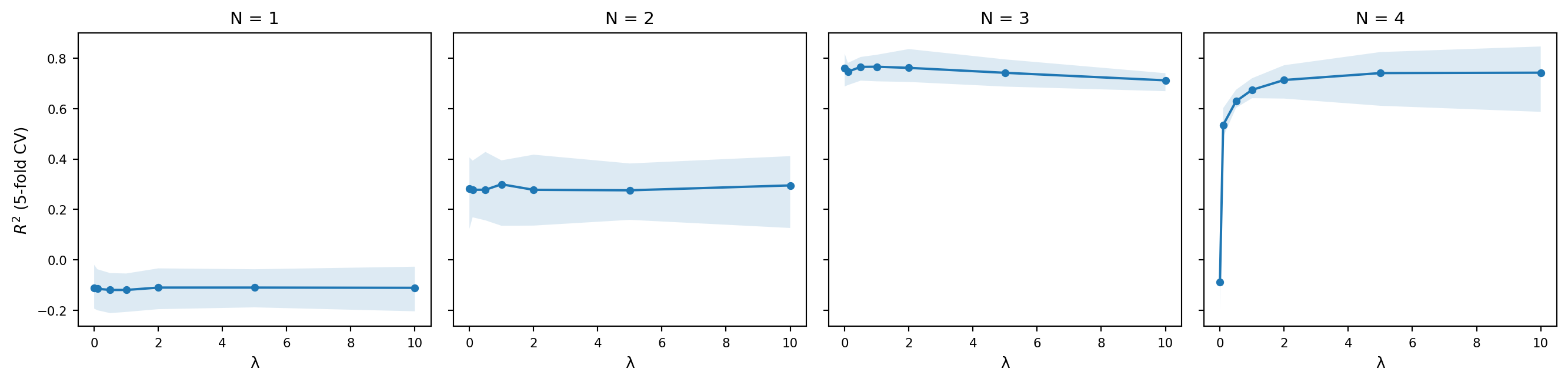
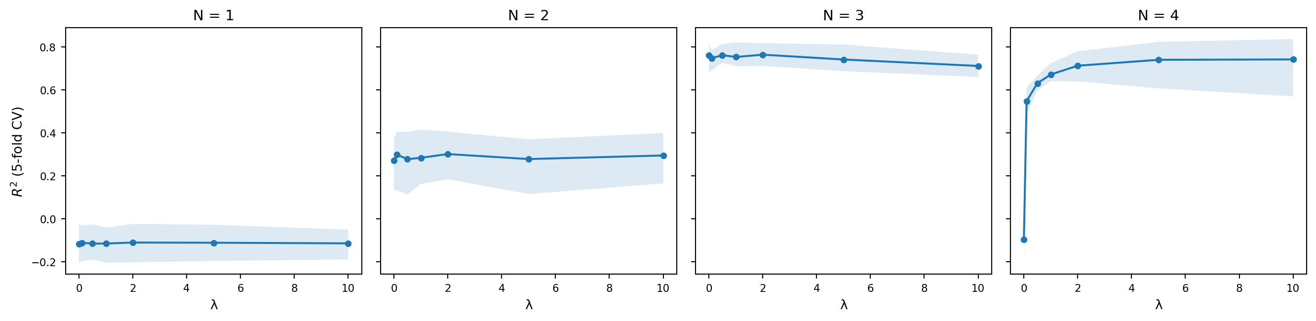
And the following plot shows the cross-validated $R^2$ as a function of $\lambda$ for each value of $N$, with bootstrap confidence intervals.
```{python}
#| code-fold: true
#| code-summary: Cross-validation performance
fig, axes = plt.subplots(1, 4, figsize=(14, 3.5), sharey=True)

for i, n in enumerate(range(1, 5)):
    ax = axes[i]
    subset = cv_stats[cv_stats.n == n]
    ax.plot(subset.lam, subset.r2, marker='o', markersize=4)
    ax.fill_between(subset.lam, subset.ci_lo, subset.ci_hi, alpha=0.15)
    ax.set_title(f'N = {n}', fontsize=11)
    ax.set_xlabel('λ', fontsize=10)
    if i == 0:
        ax.set_ylabel('$R^2$ (5-fold CV)', fontsize=10)
    ax.tick_params(labelsize=8)

fig.tight_layout()
plt.show()
```
```{python}
cv_stats.sort_values('r2', ascending=False).head(10)
```
A few things are worth noting. The unigram model ($N = 1$) does poorly regardless of $\lambda$, which makes sense: it has no way of capturing the fact that some sequences of phones are more acceptable than others, since it treats each phone independently. The bigram and trigram models do substantially better, and the best-performing models tend to use moderate smoothing. Too little smoothing and the model overfits to the training data; too much and it washes out the distinctions it learned.
A simple bigram or trigram model trained on a dictionary can predict a reasonable amount of variance in human acceptability judgments. This suggests that a good deal of phonotactic knowledge can be captured by tracking short-range sequential regularities in the lexicon, consistent with the lexicalist approach that @daland_explaining_2011 investigate.