---
title: Neighborhood density and exemplar models
bibliography: ../references.bib
jupyter: python3
---
In the [module overview](index.qmd), I described the idea of thinking about a language as a *region* around a finite set of known strings in a metric space on $\Sigma^*$. We've now built the metric—Levenshtein distance, developed in the [previous sections](levenshtein-distance.qmd)—and what remains is to define what we mean by "region." That is, given a novel string and a lexicon of known words, how do we aggregate the distances between the novel string and all the words in the lexicon into a single score that predicts how wordlike the novel string sounds?
## The Generalized Neighborhood Model
The idea that the acceptability of a string depends on its proximity to the lexicon has a long history in psycholinguistics. @luce1998recognizing proposed the *Neighborhood Activation Model* for spoken word recognition, in which the ease of recognizing a word depends on how many similar words (its "neighbors") exist in the lexicon and how frequent those neighbors are. @nosofsky1986attention developed a related framework—the *Generalized Context Model*—for categorization more broadly, in which the probability of assigning an item to a category is a function of its similarity to stored exemplars of that category.
For phonotactic acceptability, we can combine these ideas into what @daland_explaining_2011 call the *Generalized Neighborhood Model*. Given a novel string $\mathbf{w}_\text{new}$ and a lexicon of known words $\{\mathbf{w}_1, \ldots, \mathbf{w}_N\}$ with associated frequencies $\text{freq}(\mathbf{w}_j)$, the model predicts acceptability as a frequency-weighted sum of similarities:
$$\text{acceptability}(\mathbf{w}_\text{new}) = \sum_{\mathbf{w}_j \in \text{lexicon}} f_{\boldsymbol\theta}(\text{freq}(\mathbf{w}_j)) \cdot \exp\left(-\gamma \cdot \text{dist}(\mathbf{w}_j, \mathbf{w}_\text{new})\right)$$
There are several things to unpack here. The function $f_{\boldsymbol\theta}$ maps raw frequency to a weight—this allows the model to capture the fact that high-frequency neighbors might matter more (or less, or differently) than low-frequency ones. The exponential $\exp(-\gamma \cdot \text{dist}(\mathbf{w}_j, \mathbf{w}_\text{new}))$ is a *Gaussian kernel* (also called a radial basis function kernel), parameterized by a bandwidth $\gamma > 0$. It converts distance to similarity: when $\text{dist}$ is small, the exponential is close to 1 (high similarity); when $\text{dist}$ is large, the exponential is close to 0 (low similarity). The bandwidth $\gamma$ controls how quickly similarity falls off with distance.
The distance function $\text{dist}$ is where the edit distance machinery from the [previous section](levenshtein-distance.qmd) enters. We can use Levenshtein distance as $\text{dist}$—the number of insertions, deletions, and substitutions needed to transform one string into another. This gives us a concrete, computable measure of how similar a novel nonword is to each word in the lexicon.
## Computing neighborhood density
Let's implement this model and apply it to the same @daland_explaining_2011 acceptability data that we used in the [uncertainty-about-languages module](../uncertainty-about-languages/ngram-models.qmd) to evaluate $N$-gram models.
```{python}
#| code-fold: true
#| code-summary: Load data and compute edit distances
import numpy as np
import pandas as pd
import re
import nltk

nltk.download('cmudict', quiet=True)
from nltk.corpus import cmudict

# ARPABET to IPA mapping (same as in the n-gram models section)
arpabet_to_phoneme = {
    'AA': 'ɑ', 'AE': 'æ', 'AH': 'ʌ', 'AO': 'ɔ', 'AW': 'aʊ', 'AY': 'aɪ',
    'B': 'b', 'CH': 'tʃ', 'D': 'd', 'DH': 'ð', 'EH': 'ɛ', 'ER': 'ɝ',
    'EY': 'eɪ', 'F': 'f', 'G': 'g', 'HH': 'h', 'IH': 'ɪ', 'IY': 'i',
    'JH': 'dʒ', 'K': 'k', 'L': 'l', 'M': 'm', 'N': 'n', 'NG': 'ŋ',
    'OW': 'oʊ', 'OY': 'ɔɪ', 'P': 'p', 'R': 'ɹ', 'S': 's', 'SH': 'ʃ',
    'T': 't', 'TH': 'θ', 'UH': 'ʊ', 'UW': 'u', 'V': 'v', 'W': 'w',
    'Y': 'j', 'Z': 'z', 'ZH': 'ʒ'
}

# Load CMU dictionary and convert to IPA
entries = {
    word: [arpabet_to_phoneme[re.sub(r'[0-9]', '', phone)] for phone in phones]
    for word, phones in cmudict.entries()
    if len(set(word)) > 1 and len(phones) > 1 and not re.findall(r'[^a-z]', word)
}

# Load acceptability data
acceptability = pd.read_csv('../uncertainty-about-languages/Daland_etal_2011__AverageScores.csv')
acceptability['phono_cmu'] = acceptability.phono_cmu.str.strip('Coda').str.split()
acceptability['phono_ipa'] = acceptability.phono_cmu.map(
    lambda phones: [arpabet_to_phoneme[re.sub(r'[0-9]', '', p)] for p in phones]
)

print(f"Lexicon size: {len(entries)}")
print(f"Acceptability items: {len(acceptability)}")
```
Now we compute the edit distance between every nonword in the acceptability dataset and every word in the lexicon. This is computationally expensive—we're computing $|\text{lexicon}| \times |\text{nonwords}|$ edit distances—but the strings are short, so it's manageable.
```{python}
#| code-fold: true
#| code-summary: Compute edit distance matrix
def levenshtein(s, t):
    """Compute Levenshtein distance between two sequences."""
    n, m = len(s), len(t)
    dp = [[0] * (m + 1) for _ in range(n + 1)]
    for i in range(n + 1):
        dp[i][0] = i
    for j in range(m + 1):
        dp[0][j] = j
    for i in range(1, n + 1):
        for j in range(1, m + 1):
            cost = 0 if s[i-1] == t[j-1] else 1
            dp[i][j] = min(dp[i-1][j] + 1, dp[i][j-1] + 1, dp[i-1][j-1] + cost)
    return dp[n][m]


# Compute distances (this takes a moment)
nonword_phones = acceptability.phono_ipa.values
lexicon_items = list(entries.items())

# For efficiency, work with a subset of the lexicon (words with freq > threshold)
# We use all entries here since we don't have frequency data in CMUDict
distances = np.array([
    [levenshtein(phones, nw) for nw in nonword_phones]
    for _, phones in lexicon_items
])

print(f"Distance matrix shape: {distances.shape}")
print(f"Min distance: {distances.min()}, Max distance: {distances.max()}")
```
## Fitting the model
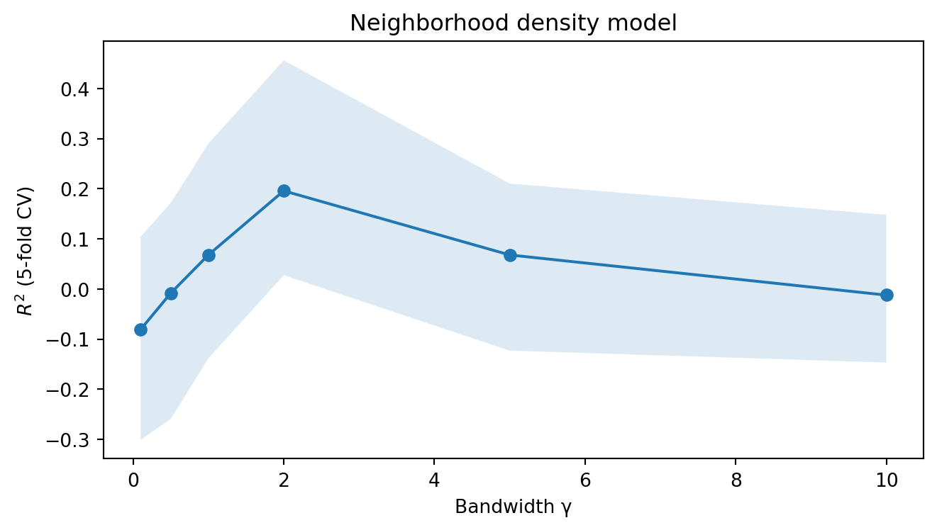
The Generalized Neighborhood Model has several hyperparameters: the bandwidth $\gamma$ of the Gaussian kernel and the parameters of the frequency weighting function $f_{\boldsymbol\theta}$. Since we don't have word frequencies from the CMU dictionary, we'll use a simplified version that treats all lexical items equally (i.e. $f_{\boldsymbol\theta}(\text{freq}) = 1$) and varies only $\gamma$.
For each value of $\gamma$, we compute the neighborhood density score for each nonword and ask how well it predicts the acceptability rating, using the same [cross-validated linear regression](../uncertainty-about-languages/ngram-models.qmd#evaluating-a-predictor) approach we used for the [$N$-gram models](../uncertainty-about-languages/ngram-models.qmd). Recall that this means fitting a linear regression on $K - 1$ folds and evaluating $R^2$ on the held-out fold, cycling through all folds and reporting the average. The bootstrap confidence intervals quantify our uncertainty about that average.
```{python}
#| code-fold: true
#| code-summary: Fit neighborhood density models
from sklearn.linear_model import LinearRegression
from sklearn.model_selection import cross_val_score
import matplotlib.pyplot as plt

gammas = [0.1, 0.5, 1.0, 2.0, 5.0, 10.0]
cv_results = []

for gamma in gammas:
    # Compute neighborhood density for each nonword
    similarities = np.exp(-gamma * distances)
    density = similarities.sum(axis=0)

    # Cross-validated regression
    scores = cross_val_score(
        LinearRegression(),
        density.reshape(-1, 1),
        acceptability.likert_rating.values,
        cv=5
    )
    stats = np.quantile(
        [np.mean(np.random.choice(scores, size=5)) for _ in range(99)],
        [0.5, 0.025, 0.975]
    )
    cv_results.append([gamma] + list(stats))

cv_results = pd.DataFrame(cv_results, columns=['gamma', 'r2', 'ci_lo', 'ci_hi'])
```
```{python}
#| code-fold: true
#| code-summary: Plot neighborhood density model performance
fig, ax = plt.subplots(1, 1, figsize=(7, 4))
ax.plot(cv_results.gamma, cv_results.r2, marker='o')
ax.fill_between(cv_results.gamma, cv_results.ci_lo, cv_results.ci_hi, alpha=0.15)
ax.set_xlabel('Bandwidth γ')
ax.set_ylabel('$R^2$ (5-fold CV)')
ax.set_title('Neighborhood density model')
fig.tight_layout()
plt.show()

cv_results
```
## Comparing the two perspectives
We can now put the two perspectives side by side. In the [uncertainty-about-languages module](../uncertainty-about-languages/ngram-models.qmd), we found that bigram and trigram models predict a substantial amount of variance in acceptability judgments. Here, we've found that neighborhood density—a measure based entirely on edit distance to the lexicon, with no probabilistic model at all—also predicts acceptability.
The question that @bailey2001determinants and @vitevitch1999probabilistic investigated is whether these two sources of information are independent or redundant. If phonotactic probability (as captured by $N$-gram models) and neighborhood density (as captured by the Generalized Neighborhood Model) make independent contributions to acceptability, then a model that uses both should outperform either alone. If they are largely redundant—if the strings that are probable under an $N$-gram model are also the strings that are close to many lexical items—then combining them will not help much.
#### Multiple regression
To test this, we extend the single-predictor [linear regression](../uncertainty-about-languages/ngram-models.qmd#evaluating-a-predictor) to [multiple regression](https://en.wikipedia.org/wiki/Multiple_regression)—a model with two predictors instead of one:
$$a_\mathbf{w} \sim \mathcal{N}(m_1 x_1 + m_2 x_2 + b, \sigma^2)$$
where $x_1$ is the log-probability from the $N$-gram model and $x_2$ is the neighborhood density score. The fitting procedure is the same as before—minimize the sum of squared residuals—but now there are two slopes to estimate. The key interpretive point is that $m_1$ captures the effect of log-probability *holding neighborhood density constant*, and $m_2$ captures the effect of neighborhood density *holding log-probability constant*. This is what it means for the two predictors to make "independent contributions": each coefficient reflects the unique predictive information carried by its predictor after accounting for the other [@hastie_elements_2009, Ch. 3].^[In the two-predictor case, if the predictors are themselves highly correlated, the individual coefficients become unstable even though the combined prediction may be fine. This phenomenon—[multicollinearity](https://en.wikipedia.org/wiki/Multicollinearity)—is not a problem for our purpose of comparing $R^2$ values, but it does mean that interpreting individual slopes requires care.]
We evaluate the combined model the same way as the individual models: cross-validated $R^2$ with bootstrap confidence intervals. If the combined $R^2$ substantially exceeds both individual values, the two predictors carry partly non-overlapping information about acceptability. If it barely exceeds the better individual model, they are largely redundant—they're capturing the same structure in the data from different angles.^[Alternatively, the increase in $R^2$ from adding a predictor can be tested with a partial $F$-test. With cross-validation, the comparison is more direct: if cross-validated $R^2$ improves when we add the second predictor, the improvement reflects out-of-sample predictive gain, not just in-sample fit.]
```{python}
#| code-fold: true
#| code-summary: Compare and combine the two approaches
from collections import defaultdict

# Load the n-gram model (refit a bigram with lambda=1)
from itertools import product

alphabet = {phone for phones in entries.values() for phone in phones}


class NgramModel:
    def __init__(self, alphabet, n=2, lam=1.0):
        self._alphabet = alphabet
        self._n = n
        self._lam = lam

    def predict(self, string):
        padded = ['<s>'] * (self._n - 1) + list(string) + ['</s>']
        logprob = 0.
        for i in range(self._n - 1, len(padded)):
            context = tuple(padded[i - self._n + 1:i])
            token = padded[i]
            if self._n == 1:
                context = ()
                if token == '<s>':
                    continue
            if context in self._logprob and token in self._logprob[context]:
                logprob += self._logprob[context][token]
            else:
                logprob += -np.inf
        return logprob

    def fit(self, lexicon):
        vocab = self._alphabet | {'</s>'}
        freq = {}
        for k in range(1, self._n):
            for ctx in product(*[self._alphabet] * (k - 1)):
                full_ctx = tuple(['<s>'] * (self._n - k)) + ctx
                freq[full_ctx] = {v: 0 for v in vocab}
        for ctx in product(*[self._alphabet] * (self._n - 1)):
            freq[ctx] = {v: 0 for v in vocab}
        if self._n == 1:
            freq[()] = {v: 0 for v in vocab}
        for word in lexicon:
            padded = ['<s>'] * (self._n - 1) + list(word) + ['</s>']
            for i in range(self._n - 1, len(padded)):
                context = tuple(padded[i - self._n + 1:i])
                token = padded[i]
                if self._n == 1:
                    context = ()
                    if token == '<s>':
                        continue
                if context in freq:
                    freq[context][token] += 1
        self._logprob = {
            ctx: {tok: np.log(count + self._lam) -
                       np.log(sum(counts.values()) + len(counts) * self._lam)
                  for tok, count in counts.items()}
            for ctx, counts in freq.items()
        }
        return self


bigram = NgramModel(alphabet, n=2, lam=1.0).fit(entries.values())
logprobs = acceptability.phono_ipa.map(bigram.predict).values
logprob_min = logprobs[logprobs != -np.inf].min()
logprobs = np.maximum(logprobs, logprob_min - 1)

# Best neighborhood density (gamma=2)
best_gamma = cv_results.loc[cv_results.r2.idxmax(), 'gamma']
similarities = np.exp(-best_gamma * distances)
density = similarities.sum(axis=0)

# Individual models
score_ngram = cross_val_score(
    LinearRegression(), logprobs.reshape(-1, 1),
    acceptability.likert_rating.values, cv=5
)
score_density = cross_val_score(
    LinearRegression(), density.reshape(-1, 1),
    acceptability.likert_rating.values, cv=5
)

# Combined model
combined = np.column_stack([logprobs, density])
score_combined = cross_val_score(
    LinearRegression(), combined,
    acceptability.likert_rating.values, cv=5
)

print(f"Bigram model R²:           {np.mean(score_ngram):.3f}")
print(f"Neighborhood density R²:   {np.mean(score_density):.3f}")
print(f"Combined model R²:         {np.mean(score_combined):.3f}")
```
The comparison tells us something about the nature of phonotactic knowledge. If the combined model substantially outperforms either individual model, it suggests that speakers' judgments are sensitive to both the sequential regularities captured by $N$-gram models and the overall similarity structure captured by neighborhood density—and that these are at least partially independent sources of information. This is broadly consistent with the findings of @vitevitch1999probabilistic, who argued that phonotactic probability and neighborhood density make separable contributions to lexical processing, and with @bailey2001determinants, who found that both factors predict wordlikeness judgments.
If the combined model does outperform either individual model, it tells us that the gradience in acceptability judgments we began investigating in the [uncertainty-about-languages module](../uncertainty-about-languages/index.qmd) reflects at least two separable sources of information: the sequential regularities that probabilistic models capture and the global similarity structure that neighborhood models capture.