from scipy.stats import rv_discreteProbability distributions
A probability distribution is a compact description of a probability space \(\langle \Omega, \mathcal{F}, \mathbb{P} \rangle\) in conjunction with a random variable whose domain is \(\Omega\) (relative to \(\mathcal{F}\)).
Discrete probability distributions
In the case of a discrete random variable \(X\) (e.g. our vowel phoneme and string-length examples), we can fully describe its probability distribution using a probability mass function (PMF) \(p_X: \text{cod}(X) \rightarrow \mathbb{R}_+\). This function is defined directly in terms of the random variable and the probability function \(\mathbb{P}\):
\[p_X(x) \equiv \mathbb{P}(\{\omega \in \Omega \mid X(\omega) = x\})\]
These definitions are related to a notation that you might be familiar with: \(\mathbb{P}(X = x) \equiv p_X(x)\). This notation is often extended to other relations \(\mathbb{P}(X \in E) = \mathbb{P}(\{\omega \in \Omega \mid \omega \in X^{-1}(E)\})\) or \(\mathbb{P}(X \leq x) \equiv \mathbb{P}(\{\omega: X(\omega) \leq x\})\).
The latter of these is often used in defining the cumulative distribution function (CDF) \(F_X: \text{cod}(X) \rightarrow \mathbb{R}_+\):
\[F_X(x) = \mathbb{P}(X \leq x) = \sum_{y \in X(\Omega):y<x} p_X(y)\]
The PMF (and by extension the CDF) is parameterized in terms of the information necessary to define their outputs for all possible inputs \(x \in X(\Omega)\). This parameterization allows us to talk about families of distributions, which all share a functional form (modulo the values of the parameters). We’ll see a few examples of this below.
In scipy, discrete distributions are implemented using scipy.rv_discrete, either by direct instantiation or subclassing.
Finite distributions
When there are a finite number of values that the random variables can take, as in the example of \(V\) above, the probability of each possibility can simply be listed. One such distribution—or really family of distributions—that we will make extensive use of—indeed, the distribution that our vowel random variable \(V\) from above has—is the categorical distribution. (It is common to talk about the categorical distribution, when we really mean the family of categorical distributions.) This distribution is parameterized by a list of probabilities \(\boldsymbol\theta\), where \(\theta_i\) gives \(p_V(i) = \mathbb{P}(V = i) = \mathbb{P}(\{\omega \in \Omega \mid V(\omega) = i\}) = \theta_i\) and \(\sum_{i \in V(\Omega)} \theta_i\).
import numpy as np

vowels = ('e', 'i', 'o', 'u', 'æ', 'ɑ', 'ɔ', 'ə', 'ɛ', 'ɪ', 'ʊ')

# this theta is totally made up
idx = np.arange(11)
theta = (0.05, 0.1, 0.1, 0.05, 0.05, 0.25, 0.15, 0.1, 0.075, 0.025, 0.05)
categorical = rv_discrete(name='categorical', values=(idx, theta))
The PMF is implemented as an instance method rv_discrete.pmf on this distribution.
import matplotlib.pyplot as plt

fig, ax = plt.subplots(1, 1)
ax.plot(list(vowels), categorical.pmf(idx), 'ro', ms=12, mec='r')
ax.vlines(list(vowels), 0, categorical.pmf(idx), colors='r', lw=4)
plt.show()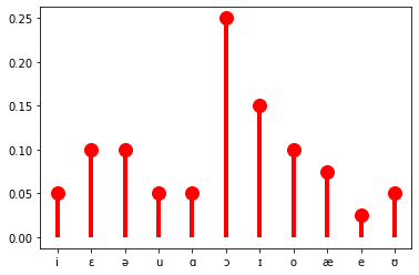
The Bernoulli distribution, which we will also make extensive use of, is a special case of the categorical distribution where \(|X(\Omega)| = 2\). By convention, \(X(\Omega) = \{0, 1\}\) In this case, we need to specify the probability \(\pi\) for only one value of \(X\), since the probability of the other must be \(1- \pi\). Indeed, more generally, we need to specify only \(|X(\Omega)| - 1\) values for a random variable \(X\) that is distributed categorical.
from scipy.stats import bernoulli

bern = bernoulli(0.25)

# annoyingly, `bernoulli.pmf` seems to be implemented
# to treat `p` as as the probability of 0
fig, ax = plt.subplots(1, 1)
ax.plot([1, 0], categorical.pmf([0, 1]), 'ro', ms=12, mec='r')
ax.vlines([1, 0], 0, categorical.pmf([0, 1]), colors='r', lw=4)
plt.show()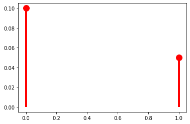
I’ll follow the convention of denoting the PMF of a particular kind of distribution using (usually shortened versions of) the distribution’s name, with the parameters following a semicolon. (The semicolon notation wil become important as we move through Module 1.)
\[\text{Cat}(x; \boldsymbol\theta) = p_X(x) = \mathbb{P}(X = x) = \mathbb{P}(\{\omega \in \Omega \mid X(\omega) = x\}) = \theta_x\]
To express the above equivalences, I’ll often write:
\[X \sim \text{Cat}(\boldsymbol{\theta})\]
This statement is read “\(X\) is distributed categorical with parameters \(\boldsymbol{\theta}\).”
So then the Bernoulli distribution would just be:
\[\text{Bern}(x; \pi) = \begin{cases}\pi & \text{if } x = 1\\1 - \pi & \text{if } x = 0\end{cases}\]
And if a random variable \(X\) is distributed Bernoulli with parameter \(\pi\), we would write:
\[X \sim \text{Bern}(\pi)\]
It’s sometimes useful to write the PMF for the categorical and Bernoulli distributions as:
\[\text{Cat}(x; \boldsymbol\theta) = \prod_{i \in V(\Omega)} \theta_i^{1_{\{x\}}[i]}\]
\[\text{Bern}(x; \pi) = \pi^{x}(1-\pi)^{1-x}\]
where
\[1_A[x] = \begin{cases}1 & \text{if } x \in A\\ 0 & \text{otherwise}\\ \end{cases}\]
In an abuse of notation, I will sometimes write:
\[\text{Cat}(x; \boldsymbol\theta) = \prod_{i \in V(\Omega)} \theta_i^{1_{x}[i]}\]
Categorical and Bernoulli distributions won’t be the only finite distributions we work with, but they will be the most common.
Countably infinite distributions
When there are a countably infinite number of values that a random variable can take, as in the example of string length \(L\) above, the probability of each possibility cannot simply be listed: we need some way of computing it for any value.
However we compute these values, they must sum to one as required by the assumption of unit measure: \(\mathbb{P}(\Omega) = 1\). Since \(\mathbb{P}(\Omega) = \sum_{x \in X(\Omega)} p_X(x)\), another way of stating this requirement is to say that the series \(\sum_{x \in X(\Omega)} p_X(x)\) must converge to 1.
One example of such a series is a geometric series, such as \(\sum_{k=1}^\infty \frac{1}{2^k} = \frac{1}{2} + \frac{1}{4} + \frac{1}{8} + \ldots = 1\). This series gives us our first example of a probability distribution with infinite support–i.e. one that assigns a non-zero probability to an infinite (but countable) number of values of a random variable. So for instance, if we are considering our random variable \(L\) mapping strings to their lengths, \(p_X(k) = \frac{1}{2^k}\) is a possible PMF for \(L\). (This assumes that strings cannot have zero length, meaning that \(\Omega = \Sigma^+\) rather than \(\Sigma^*\); if we want to allow zero-length strings \(\epsilon\), we would need \(p_X(k) = \frac{1}{2^{k+1}}\).)
class parameterless_geometric_gen(rv_discrete):
    "A special case of the geometric distribution without parameters"
    def _pmf(self, k):
        return 2.0 ** -(k+1)

parameterless_geometric = parameterless_geometric_gen(name="parameterless_geometric")

k = np.arange(10)

fig, ax = plt.subplots(1, 1)
ax.plot(k, parameterless_geometric.pmf(k), 'ro', ms=12, mec='r')
ax.vlines(k, 0, parameterless_geometric.pmf(k), colors='r', lw=4)
plt.show()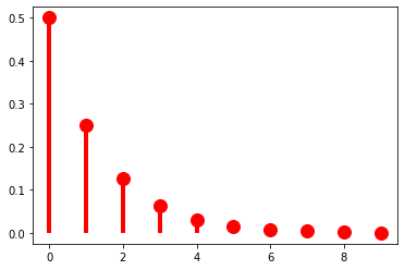
As it stands, this distribution has no parameters, meaning that we have no control over how quickly the probabilities drop off. The geometric distribution provides us this control using a parameter to \(\pi \in (0, 1]\):
\[\text{Geom}(x; \pi) = (1-\pi)^k\pi\]
When \(\pi = \frac{1}{2}\), we get exactly the distribution above.
from scipy.stats import geom

p = 0.5

fig, ax = plt.subplots(1, 1)
ax.plot(k, geom(p).pmf(k+1), 'ro', ms=12, mec='r')
ax.vlines(k, 0, geom(p).pmf(k+1), colors='r', lw=4)
plt.show()
As \(\pi \rightarrow 0\), the distribution flattens out (or becomes denser).
p = 0.1

fig, ax = plt.subplots(1, 1)
ax.plot(k, geom(p).pmf(k+1), 'ro', ms=12, mec='r')
ax.vlines(k, 0, geom(p).pmf(k+1), colors='r', lw=4)
plt.show()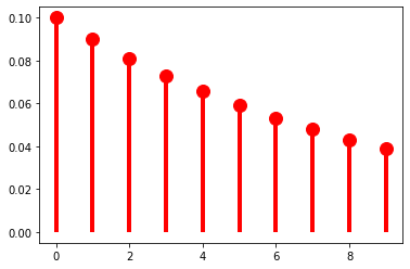
And as \(\pi \rightarrow 1\), it becomes sharper (or sparser).
p = 0.9

fig, ax = plt.subplots(1, 1)
ax.plot(k, geom(p).pmf(k+1), 'ro', ms=12, mec='r')
ax.vlines(k, 0, geom(p).pmf(k+1), colors='r', lw=4)
plt.show()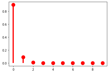
At this point, it’s useful to pause for a moment to think about what exactly a parameter like \(\pi\) is. I said above that random variables and probability distributions together provide a way of classifying probability spaces: in saying that \(p_X(k) = (1-\pi)^k\pi\) we are describing \(\mathbb{P}: \mathcal{F} \rightarrow \mathbb{R}_+\) by using \(X\) to abstract across whatever the underlying measurable space \(\langle \Omega, \mathcal{F} \rangle\) is. The distribution gives you the form of that description; the parameter \(\pi\) gives the content of the description. Because the use of \(X\) is always implied, unless it really matters, I’m going to start dropping \(X\) from \(p_X\) unless I’m emphasizing the random variable in some way.
The \(\pi\) parameter of a geometric distribution allows us to describe distributions that have a very particular shape–namely, ones where \(\forall k \in \mathbb{N}: p(k) > p(k + 1)\). But this isn’t always a good way of describing a particular distribution. For instance, for our string-length variable \(L\), it’s probably a pretty bad description regardless of what particular distribution on string lengths (type or token) we’re describing because 1 grapheme/phoneme words just aren’t more frequent than two grapheme/phoneme words. This point can be seen if we look at the distribution of word lengths at the type level in the CMU Pronouncing Dictionary, which contains phonemic transcriptions of English words and which we’ll use extensively in Module 2.
from urllib.request import urlopen

cmudict_url = "http://svn.code.sf.net/p/cmusphinx/code/trunk/cmudict/cmudict-0.7b"

with urlopen(cmudict_url) as cmudict:
  words = [
      line.split()[1:] for line in cmudict if line[0] != 59
  ]

_ = plt.hist([len(w) for w in words], bins=32)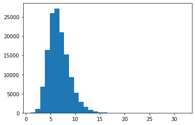
One such distribution that give us more flexibility in this respect is the negative binomial distribution, which is a very useful for modeling token frequency in text (Church and Gale 1995). This distribution effectively generalizes the geometric by allowing us to control the exponent on \(\pi\) with a new parameter \(r\).
\[\text{NegBin}(k; \pi, r) = {k+r-1 \choose r-1}(1-\pi)^{k}\pi^{r}\]
This added flexibility in turn requires us to add an additional term \({k+r-1 \choose r-1} = \frac{(k+r-1)!}{(r-1)!\,(k)!}\) that ensures that the series \(\sum_{k=0}^\infty \text{NegBin}(k; \pi, r)\) converges to \(1\). The pieces of this term that do not include the value we’re computing the probability of–i.e. \(\frac{1}{(r-1)!}\)–are often called the normalizing constant. We will make extensive use of this concept as the course moves forward.
When \(r = 1\), we of course just get the geometric distribution. As such, if we keep \(r = 1\), manipulating \(\pi\) will have the same effect we saw above.
from scipy.stats import nbinom

p = 0.5
r = 1

fig, ax = plt.subplots(1, 1)
ax.plot(k, nbinom(r, p).pmf(k+1), 'ro', ms=12, mec='r')
ax.vlines(k, 0, nbinom(r, p).pmf(k+1), colors='r', lw=4)
plt.show()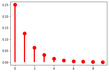
As \(r\) grows, though, we get very different behavior: \(p(k)\) is no longer always greater than \(p(k + 1)\). Another way of saying this is that we can use \(r\) to shift the probability mass rightward.
p = 0.5
r = 5

fig, ax = plt.subplots(1, 1)
ax.plot(k, nbinom(r, p).pmf(k+1), 'ro', ms=12, mec='r')
ax.vlines(k, 0, nbinom(r, p).pmf(k+1), colors='r', lw=4)
plt.show()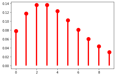
The mass-shifting effect is modulated by \(\pi\): it accelerates with small \(\pi\)…
p = 0.1
r = 5

fig, ax = plt.subplots(1, 1)
ax.plot(k, nbinom(r, p).pmf(k+1), 'ro', ms=12, mec='r')
ax.vlines(k, 0, nbinom(r, p).pmf(k+1), colors='r', lw=4)
plt.show()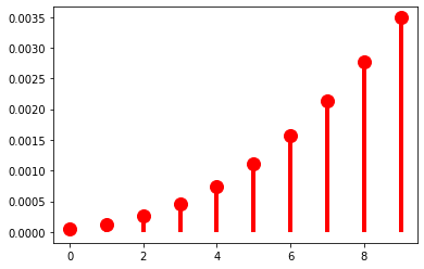
…but decelerates with large \(\pi\).
p = 0.9
r = 5

fig, ax = plt.subplots(1, 1)
ax.plot(k, nbinom(r, p).pmf(k+1), 'ro', ms=12, mec='r')
ax.vlines(k, 0, nbinom(r, p).pmf(k+1), colors='r', lw=4)
plt.show()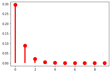
p = 0.9
r = 40

fig, ax = plt.subplots(1, 1)
ax.plot(k, nbinom(r, p).pmf(k+1), 'ro', ms=12, mec='r')
ax.vlines(k, 0, nbinom(r, p).pmf(k+1), colors='r', lw=4)
plt.show()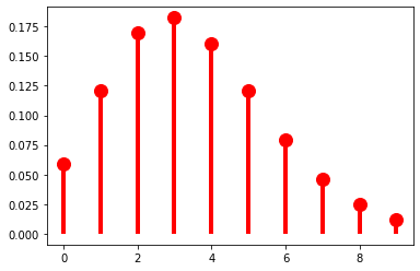
We won’t talk about how to fit a distribution to some data until later, when we talk about parameter estimation; but the negative binomial distribution can provide a reasonably good description of the empirical distribution of word lengths. One way to visualize this is to compare the empirical CDF with the CDF of the best fitting negative binomial.
from statsmodels.distributions.empirical_distribution import ECDF
from statsmodels.discrete.discrete_model import NegativeBinomial

ecdf = ECDF([len(w) for w in words])
negbin_fit = NegativeBinomial([len(w) for w in words], np.ones(len(words))).fit()

p = 1/np.exp(1+negbin_fit.params[0]*negbin_fit.params[1])
r = np.exp(negbin_fit.params[0])*p/(1-p)

print(f"p = {np.round(p, 2)}, r = {np.round(r, 2)}")

k = np.arange(30)

fig, ax = plt.subplots(1, 1)
plt.plot(np.mgrid[1:30:0.1], ecdf(np.mgrid[1:30:0.1]))
plt.plot(np.mgrid[1:30:0.1], nbinom(r, p).cdf(np.mgrid[1:30:0.1]))
plt.show()
Optimization terminated successfully.
Current function value: 2.180477
Iterations: 23
Function evaluations: 25
Gradient evaluations: 25
p = 0.37, r = 3.71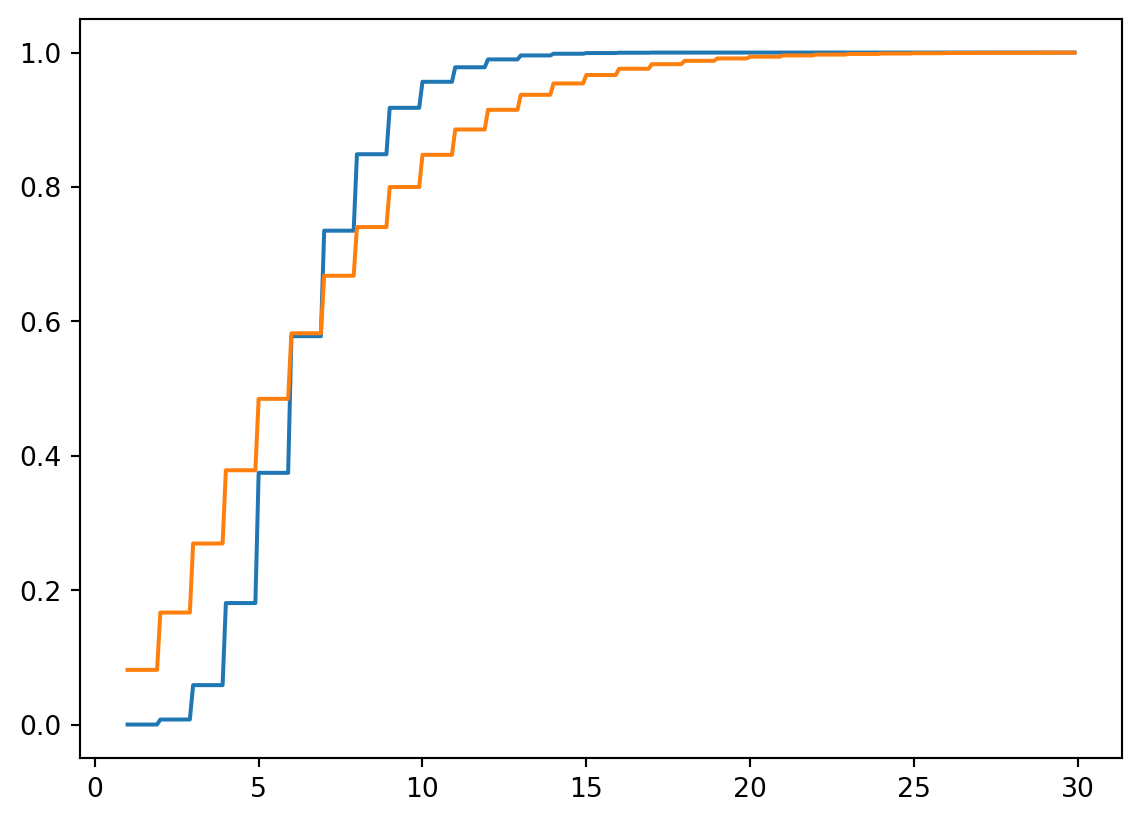
A limiting case of the negative binomial distribution that you may be familiar with is the Poisson distribution.
\[\text{Pois}(k; \lambda) = \frac{\lambda^k\exp(-\lambda)}{k!}\]
The Poisson distribution arises as \(\text{Pois}(k; \lambda) = \lim_{r \rightarrow \infty} \text{NegBin} \left(k; r, \frac{\lambda}{r + \lambda}\right)\).
Continuous probability distributions
Continuous random variables—those whose range is uncountable, like formant values—require a different tool: a probability density function (PDF) rather than a PMF. The key difference is that a PDF does not give you the probability of a particular value (which is always zero for a continuous random variable); rather, the probability that the variable falls in some interval is the integral of the PDF over that interval. Common continuous distributions include the uniform, beta, and Gaussian (normal) distributions.
Since the language models we’ll work with in this course operate over discrete symbol sequences, we won’t need continuous distributions here. But they will come up later—for instance, when we discuss parameter estimation—and the Wikipedia articles linked above are a good starting point if you want to read ahead.
References
Church, Kenneth W., and William A. Gale. 1995. “Poisson Mixtures.” Natural Language Engineering 1 (2): 163–90. https://doi.org/10.1017/S1351324900000139.